3. Machine Learning Models
Machine learning (ML) is a subfield of artificial intelligence (AI) focused on developing algorithms and statistical models that enable computers to learn from and make decisions based on data. Unlike traditional programming, where explicit instructions are given, machine learning systems identify patterns and insights from large datasets, improving their performance over time through experience.
ML encompasses various techniques, including supervised learning, where models are trained on labeled data to predict outcomes; unsupervised learning, which involves discovering hidden patterns or groupings within unlabeled data; and reinforcement learning, where models learn optimal actions through trial and error in dynamic environments. These methods are applied across diverse domains, from natural language processing and computer vision to recommendation systems and autonomous vehicles, revolutionizing how technology interacts with the world.
3.1 Decision Tree and Random Forest
3.1.1 Decision Trees
Decision Trees are intuitive and powerful models used in machine learning to make predictions and decisions. Think of it like playing a game of 20 questions, where each question helps you narrow down the possibilities. Decision trees function similarly; they break down a complex decision into a series of simpler questions based on the data.
Each question, referred to as a “decision,” relies on a specific characteristic or feature of the data. For instance, if you’re trying to determine whether a fruit is an apple or an orange, the initial question might be, “Is the fruit’s color red or orange?” Depending on the answer, you might follow up with another question—such as, “Is the fruit’s size small or large?” This questioning process continues until you narrow it down to a final answer (e.g., the fruit is either an apple or an orange).
In a decision tree, these questions are represented as nodes, and the possible answers lead to different branches. The final outcomes are represented at the end of each branch, known as leaf nodes. One of the key advantages of decision trees is their clarity and ease of understanding—much like a flowchart. However, they can also be prone to overfitting, especially when dealing with complex datasets that have many features. Overfitting occurs when a model performs exceptionally well on training data but fails to generalize to new or unseen data.
In summary, decision trees offer an intuitive approach to making predictions and decisions, but caution is required to prevent them from becoming overly complicated and tailored too closely to the training data.
3.1.2 Random Forest
Random Forests address the limitations of decision trees by utilizing an ensemble of multiple trees instead of relying on a single one. Imagine you’re gathering opinions about a game outcome from a group of people; rather than trusting just one person’s guess, you ask everyone and then take the most common answer. This is the essence of how a Random Forest operates.
In a Random Forest, numerous decision trees are constructed, each making its own predictions. However, a key difference is that each tree is built using a different subset of the data and considers different features of the data. This technique, known as bagging (Bootstrap Aggregating), allows each tree to provide a unique perspective, which collectively leads to a more reliable prediction.
When making a final prediction, the Random Forest aggregates the predictions from all the trees. For classification tasks, it employs majority voting to determine the final class label, while for regression tasks, it averages the results.
Random Forests typically outperform individual decision trees because they are less likely to overfit the data. By combining multiple trees, they achieve a balance between model complexity and predictive performance on unseen data.
Real-Life Analogy
Consider Andrew, who wants to decide on a destination for his year-long vacation. He starts by asking his close friends for suggestions. The first friend asks Andrew about his past travel preferences, using his answers to recommend a destination. This is akin to a decision tree approach—one friend following a rule-based decision process.
Next, Andrew consults more friends, each of whom poses different questions to gather recommendations. Finally, Andrew chooses the places suggested most frequently by his friends, mirroring the Random Forest algorithm’s method of aggregating multiple decision trees’ outputs.
3.1.3 Implementing Random Forest on the BBBP Dataset
This guide demonstrates how to implement a Random Forest algorithm in Python using the BBBP (Blood–Brain Barrier Permeability) dataset. The BBBP dataset is used in cheminformatics to predict whether a compound can cross the blood-brain barrier based on its chemical structure.
The dataset contains SMILES (Simplified Molecular Input Line Entry System) strings representing chemical compounds, and a target column that indicates whether the compound is permeable to the blood-brain barrier or not.
The goal is to predict whether a given chemical compound will cross the blood-brain barrier, based on its molecular structure. This guide walks you through downloading the dataset, processing it, and training a Random Forest model.
Step 1: Install RDKit (Required for SMILES to Fingerprint Conversion)
We need to use the RDKit library, which is essential for converting SMILES strings into molecular fingerprints, a numerical representation of the molecule.
# Install the RDKit package via conda-forge
!pip install -q condacolab
import condacolab
condacolab.install()

# Now install RDKit
!mamba install -c conda-forge rdkit -y

# Import RDKit and check if it's installed successfully
from rdkit import Chem
print("RDKit is successfully installed!")
Step 2: Download the BBBP Dataset from Kaggle
The BBBP dataset is hosted on Kaggle, a popular platform for datasets and machine learning competitions. To access the dataset, you need a Kaggle account and an API key for authentication. Here’s how you can set it up:
Step 2.1: Create a Kaggle Account
- Visit Kaggle and create an account if you don’t already have one.
- Once you’re logged in, go to your profile by clicking on your profile picture in the top right corner, and select My Account.
Step 2.2: Set Up the Kaggle API Key
- Scroll down to the section labeled API on your account page.
- Click on the button “Create New API Token”. This will download a file named kaggle.json to your computer.
- Keep this file safe! It contains your API key, which you’ll use to authenticate when downloading datasets.
Step 2.3: Upload the Kaggle API Key
Once you have the kaggle.json file, you need to upload it to your Python environment:
- If you’re using a notebook environment like Google Colab, use the code below to upload the file:
# Upload the kaggle.json file from google.colab import
files uploaded = files.upload()
# Move the file to the right directory for authentication
!mkdir -p ~/.kaggle !mv kaggle.json ~/.kaggle/ !chmod 600 ~/.kaggle/kaggle.json
- If you’re using a local Jupyter Notebook:
Place the kaggle.json file in a folder named .kaggle within your home directory:
- On Windows: Place it in C:\Users<YourUsername>.kaggle.
- On Mac/Linux: Place it in ~/.kaggle.
Step 2.4: Install the Required Libraries
To interact with Kaggle and download the dataset, you need the Kaggle API client. Install it with the following command:
!pip install kaggle
Step 2.5: Download the BBBP Dataset
Now that the API key is set up, you can download the dataset using the Kaggle API:
# Download the BBBP dataset using the Kaggle API
!kaggle datasets download -d priyanagda/bbbp-smiles
# Unzip the downloaded file
!unzip bbbp-smiles.zip -d bbbp_dataset
This code will:
- Download the dataset into your environment.
- Extract the dataset files into a folder named bbbp_dataset.
Step 2.6: Verify the Download
After downloading, check the dataset files to confirm that everything is in place:
# List the files in the dataset folder
import os
dataset_path = "bbbp_dataset"
files = os.listdir(dataset_path)
print("Files in the dataset:", files)
By following these steps, you will have successfully downloaded and extracted the BBBP dataset, ready for further analysis and processing.
Step 3: Load the BBBP Dataset
After downloading the dataset, we’ll load the BBBP dataset into a pandas DataFrame. The dataset contains the SMILES strings and the target variable (p_np), which indicates whether the compound can cross the blood-brain barrier (binary classification: 1 for permeable, 0 for non-permeable).
import pandas as pd

# Load the BBBP dataset (adjust the filename if it's different)
data = pd.read_csv("bbbp.csv")  # Assuming the dataset is named bbbp.csv
print("Dataset Head:", data.head())
Step 4: Convert SMILES to Molecular Fingerprints
To use the SMILES strings for modeling, we need to convert them into molecular fingerprints. This process turns the chemical structures into a numerical format that can be fed into machine learning models. We’ll use RDKit to generate these fingerprints using the Morgan Fingerprint method.
from rdkit import Chem
from rdkit.Chem import AllChem
import numpy as np

# Function to convert SMILES to molecular fingerprints
def featurize_molecule(smiles):
    mol = Chem.MolFromSmiles(smiles)
    if mol:
        return AllChem.GetMorganFingerprintAsBitVect(mol, 2, nBits=1024)
    else:
        return None

# Apply featurization to the dataset
features = [featurize_molecule(smi) for smi in data['smiles']]  # Replace 'smiles' with the actual column name if different
features = [list(fp) if fp is not None else np.zeros(1024) for fp in features]  # Handle missing data by filling with zeros
X = np.array(features)
y = data['p_np']  # Target column (1 for permeable, 0 for non-permeable)
The diagram below provides a visual representation of what this code does:
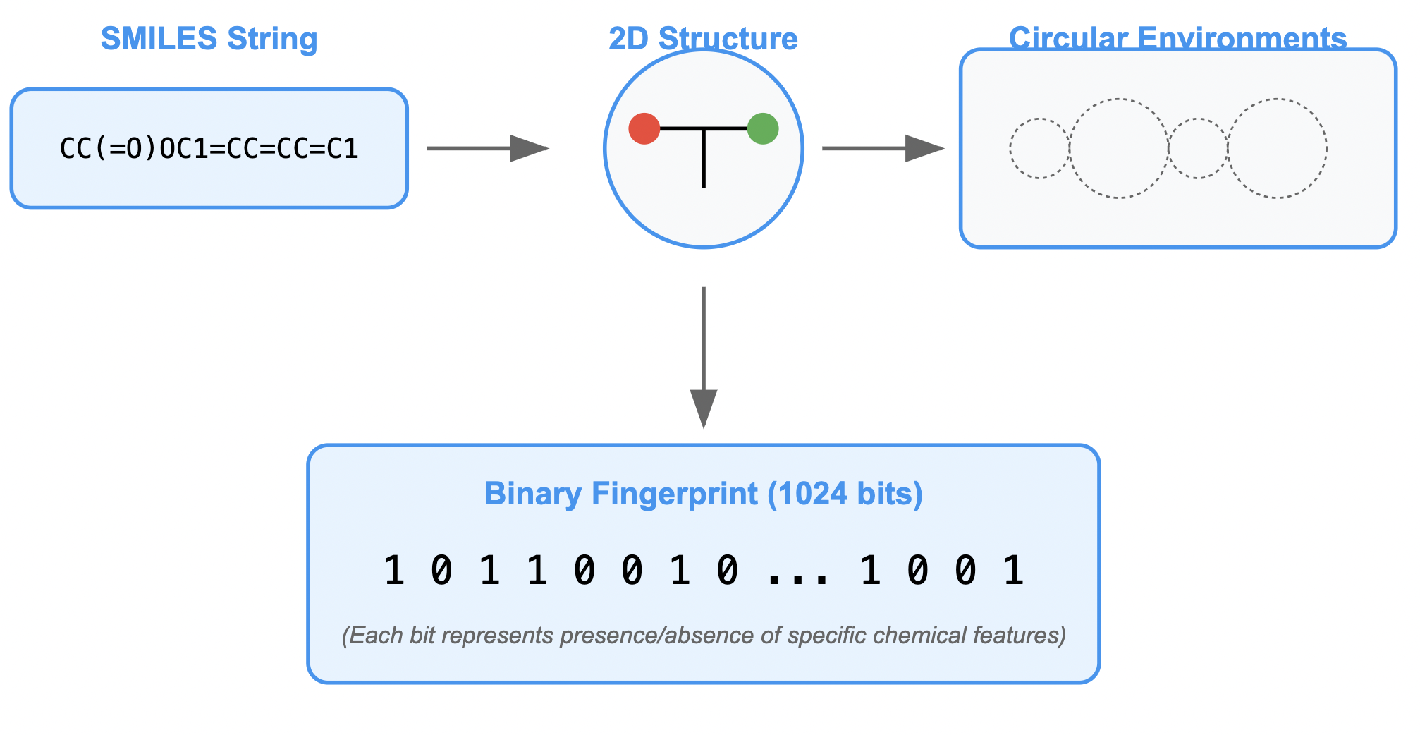
Figure: SMILES to Molecular Fingerprints Conversion Process
Step 5: Split Data into Training and Testing Sets
To evaluate the model, we need to split the data into training and testing sets. The train_test_split function from scikit-learn will handle this. We’ll use 80% of the data for training and 20% for testing.
from sklearn.model_selection import train_test_split

# Split data into train and test sets (80% training, 20% testing)
X_train, X_test, y_train, y_test = train_test_split(X, y, test_size=0.2, random_state=42)
The diagram below provides a visual representation of what this code does:
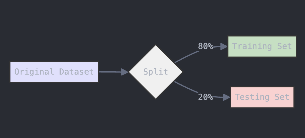
Figure: Data Splitting Process for Training and Testing
Step 6: Train the Random Forest Model
We’ll use the RandomForestClassifier from scikit-learn to build the model. A Random Forest is an ensemble method that uses multiple decision trees to make predictions. The more trees (n_estimators) we use, the more robust the model will be, but the longer the model will take to run. For the most part, n_estimators is set to 100 in most versions of scikit-learn. However, for more complex datasets, higher values like 500 or 1000 may improve performance.
from sklearn.ensemble import RandomForestClassifier

# Train a Random Forest classifier
rf_model = RandomForestClassifier(n_estimators=100, random_state=42)
rf_model.fit(X_train, y_train)
The diagram below provides a visual explanation of what is going on here:
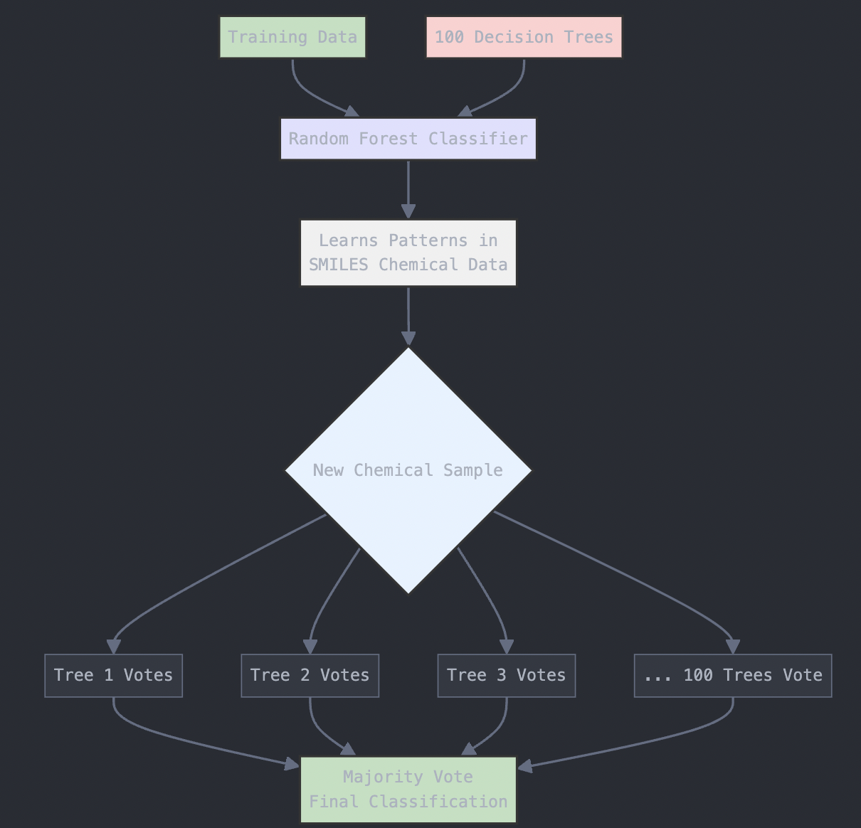
Figure: Random Forest Algorithm Structure
Step 7: Evaluate the Model
After training the model, we’ll use the test data to evaluate its performance. We will print the accuracy and the classification report to assess the model’s precision, recall, and F1 score.
from sklearn.metrics import accuracy_score, classification_report

# Predictions on the test set
y_pred = rf_model.predict(X_test)

# Evaluate accuracy and performance
accuracy = accuracy_score(y_test, y_pred)
print("Accuracy:", accuracy)
print("Classification Report:", classification_report(y_test, y_pred))
Model Performance and Parameters
- Accuracy: The proportion of correctly predicted instances out of all instances.
- Classification Report: Provides additional metrics like precision, recall, and F1 score.
In this case, we achieved an accuracy score of ~87%.
Key Hyperparameters:
- n_estimators: The number of trees in the Random Forest. More trees generally lead to better performance but also require more computational resources.
- test_size: The proportion of data used for testing. A larger test size gives a more reliable evaluation but reduces the amount of data used for training.
- random_state: Ensures reproducibility by initializing the random number generator to a fixed seed.
Conclusion
This guide demonstrated how to implement a Random Forest model to predict the Blood–Brain Barrier Permeability (BBBP) using the BBBP dataset. By converting SMILES strings to molecular fingerprints and using a Random Forest classifier, we were able to achieve an accuracy score of around 87%.
Adjusting parameters like the number of trees (n_estimators) or the split ratio (test_size) can help improve the model’s performance. Feel free to experiment with these parameters and explore other machine learning models for this task!
3.1.4 Approaching Random Forest Problems
When tackling a classification or regression problem using the Random Forest algorithm, a systematic approach can enhance your chances of success. Here’s a step-by-step guide to effectively solve any Random Forest problem:
-
Understand the Problem Domain: Begin by thoroughly understanding the problem you are addressing. Identify the nature of the data and the specific goal—whether it’s classification (e.g., predicting categories) or regression (e.g., predicting continuous values). Familiarize yourself with the dataset, including the features (independent variables) and the target variable (dependent variable).
-
Data Collection and Preprocessing: Gather the relevant dataset and perform necessary preprocessing steps. This may include handling missing values, encoding categorical variables, normalizing or standardizing numerical features, and removing any outliers. Proper data cleaning ensures that the model learns from quality data.
-
Exploratory Data Analysis (EDA): Conduct an exploratory data analysis to understand the underlying patterns, distributions, and relationships within the data. Visualizations, such as scatter plots, histograms, and correlation matrices, can provide insights that inform feature selection and model tuning.
-
Feature Selection and Engineering: Identify the most relevant features for the model. This can be achieved through domain knowledge, statistical tests, or feature importance metrics from preliminary models. Consider creating new features through feature engineering to enhance model performance.
-
Model Training and Parameter Tuning: Split the dataset into training and testing sets, typically using an 80-20 or 70-30 ratio. Train the Random Forest model using the training data, adjusting parameters such as the number of trees (
n_estimators), the maximum depth of the trees (max_depth), and the minimum number of samples required to split an internal node (min_samples_split). Utilize techniques like grid search or random search to find the optimal hyperparameters. -
Model Evaluation: Once trained, evaluate the model’s performance on the test set using appropriate metrics. For classification problems, metrics such as accuracy, precision, recall, F1 score, and ROC-AUC are valuable. For regression tasks, consider metrics like mean absolute error (MAE), mean squared error (MSE), and R-squared.
-
Interpretation and Insights: Analyze the model’s predictions and feature importance to derive actionable insights. Understanding which features contribute most to the model can guide decision-making and further improvements in the model or data collection.
-
Iterate and Improve: Based on the evaluation results, revisit the previous steps to refine your model. This may involve further feature engineering, collecting more data, or experimenting with different algorithms alongside Random Forest to compare performance.
-
Deployment: Once satisfied with the model’s performance, prepare it for deployment. Ensure the model can process incoming data and make predictions in a real-world setting, and consider implementing monitoring tools to track its performance over time.
By following this structured approach, practitioners can effectively leverage the Random Forest algorithm to solve a wide variety of problems, ensuring thorough analysis, accurate predictions, and actionable insights.
3.1.5 Strengths and Weaknesses of Random Forest
Strengths:
-
Robustness: Random Forests are less prone to overfitting compared to individual decision trees, making them more reliable for new data.
-
Versatility: They can handle both classification and regression tasks effectively.
-
Feature Importance: Random Forests provide insights into the significance of each feature in making predictions.
Weaknesses:
-
Complexity: The model can become complex, making it less interpretable than single decision trees.
-
Resource Intensive: Training a large number of trees can require significant computational resources and time.
-
Slower Predictions: While individual trees are quick to predict, aggregating predictions from multiple trees can slow down the prediction process.
Section 3.1 – Quiz Questions
1) Factual Questions
Question 1
What is the primary reason a Decision Tree might perform very well on training data but poorly on new, unseen data?
A. Underfitting
B. Data leakage
C. Overfitting
D. Regularization
▶ Click to show answer
Correct Answer: C▶ Click to show explanation
Explanation: Decision Trees can easily overfit the training data by creating very complex trees that capture noise instead of general patterns. This hurts their performance on unseen data.Question 2
In a Decision Tree, what do the internal nodes represent?
A. Possible outcomes
B. Splitting based on a feature
C. Aggregation of multiple trees
D. Random subsets of data
▶ Click to show answer
Correct Answer: B▶ Click to show explanation
Explanation: Internal nodes represent decision points where the dataset is split based on the value of a specific feature (e.g., "Is the fruit color red or orange?").Question 3
Which of the following best explains the Random Forest algorithm?
A. A single complex decision tree trained on all the data
B. Many decision trees trained on identical data to improve depth
C. Many decision trees trained on random subsets of the data and features
D. A clustering algorithm that separates data into groups
▶ Click to show answer
Correct Answer: C▶ Click to show explanation
Explanation: Random Forests use bagging to train multiple decision trees on different random subsets of the data and different random subsets of features, making the ensemble more robust.Question 4
When training a Random Forest for a classification task, how is the final prediction made?
A. By taking the median of the outputs
B. By taking the average of probability outputs
C. By majority vote among trees’ predictions
D. By selecting the tree with the best accuracy
▶ Click to show answer
Correct Answer: C▶ Click to show explanation
Explanation: For classification problems, the Random Forest algorithm uses majority voting — the class most predicted by the individual trees becomes the final prediction.2) Conceptual Questions
Question 5
You are given a dataset containing information about chemical compounds, with many categorical features (such as “molecular class” or “bond type”).
Would using a Random Forest model be appropriate for this dataset?
A. No, Random Forests cannot handle categorical data.
B. Yes, Random Forests can naturally handle datasets with categorical variables after encoding.
C. No, Random Forests only work on images.
D. Yes, but only if the dataset has no missing values.
▶ Click to show answer
Correct Answer: B▶ Click to show explanation
Explanation: Random Forests can handle categorical data after simple preprocessing, such as label encoding or one-hot encoding. They are robust to different feature types, including numerical and categorical.Question 6
Suppose you have your molecule fingerprints stored in variables X and your labels (0 or 1 for BBBP) stored in y.
Which of the following correctly splits the data into 80% training and 20% testing sets?
A.
X_train, X_test, y_train, y_test = train_test_split(X, y, train_size=0.2, random_state=42)
B.
X_train, X_test, y_train, y_test = train_test_split(X, y, test_size=0.2, random_state=42)
C.
X_train, X_test = train_test_split(X, y, test_size=0.8, random_state=42)
D.
X_train, y_train, X_test, y_test = train_test_split(X, y, test_size=0.2, random_state=42)
▶ Click to show answer
Correct Answer: B▶ Click to show explanation
Explanation: In Random Forest modeling, we use train_test_split from sklearn.model_selection. test_size=0.2 reserves 20% of the data for testing, leaving 80% for training. The function returns train features, test features, train labels, and test labels — in that exact order: X_train, X_test, y_train, y_test = train_test_split(X, y, test_size=0.2, random_state=42) A, C, and D are wrong because... (A) reverses train and test sizing. (C) mistakenly sets test_size=0.8 (which would leave only 20% for training — wrong). (D) messes up the return order (train features and labels must come first).▶ Show Solution Code
from sklearn.model_selection import train_test_split

X_train, X_test, y_train, y_test = train_test_split(X, y, test_size=0.2, random_state=42)
3.2 Neural Network
A neural network is a computational model inspired by the neural structure of the human brain, designed to recognize patterns and learn from data. It consists of layers of interconnected nodes, or neurons, which process input data through weighted connections.
Structure: Neural networks typically include an input layer, one or more hidden layers, and an output layer. Each neuron in a layer is connected to neurons in the adjacent layers. The input layer receives data, the hidden layers transform this data through various operations, and the output layer produces the final prediction or classification.
Functioning: Data is fed into the network, where each neuron applies an activation function to its weighted sum of inputs. These activation functions introduce non-linearity, allowing the network to learn complex patterns. The output of the neurons is then passed to the next layer until the final prediction is made.
Learning Process: Neural networks learn through a process called training. During training, the network adjusts the weights of connections based on the error between its predictions and the actual values. This is achieved using algorithms like backpropagation and optimization techniques such as gradient descent, which iteratively updates the weights to minimize the prediction error.
3.2.1 Biological and Conceptual Foundations of Neural Networks
Neural networks are a class of machine learning models designed to learn patterns from data in order to make predictions or classifications. Their structure and behavior are loosely inspired by how the human brain processes information: through a large network of connected units that transmit signals to each other. Although artificial neural networks are mathematical rather than biological, this analogy provides a helpful starting point for understanding how they function.
The Neural Analogy
In a biological system, neurons receive input signals from other neurons, process those signals, and send output to downstream neurons. Similarly, an artificial neural network is composed of units called “neurons” or “nodes” that pass numerical values from one layer to the next. Each of these units receives inputs, processes them using a simple rule, and forwards the result.
This structure allows the network to build up an understanding of the input data through multiple layers of transformations. As information flows forward through the network—layer by layer—it becomes increasingly abstract. Early layers may focus on basic patterns in the input, while deeper layers detect more complex or chemically meaningful relationships.
Layers of a Neural Network
Neural networks are organized into three main types of layers:
- Input Layer: This is where the network receives the data. In chemistry applications, this might include molecular fingerprints, structural descriptors, or other numerical representations of a molecule.
- Hidden Layers: These are the internal layers where computations happen. The network adjusts its internal parameters to best relate the input to the desired output.
- Output Layer: This layer produces the final prediction. For example, it might output a predicted solubility value, a toxicity label, or the probability that a molecule is biologically active.
The depth (number of layers) and width (number of neurons in each layer) of a network affect its capacity to learn complex relationships.
Why Chemists Use Neural Networks
Many molecular properties—such as solubility, lipophilicity, toxicity, and biological activity—are influenced by intricate, nonlinear combinations of atomic features and substructures. These relationships are often difficult to express with a simple equation or rule.
Neural networks are especially useful in chemistry because:
- They can learn from large, complex datasets without needing detailed prior knowledge about how different features should be weighted.
- They can model nonlinear relationships, such as interactions between molecular substructures, electronic effects, and steric hindrance.
- They are flexible and can be applied to a wide range of tasks, from predicting reaction outcomes to screening drug candidates.
How Learning Happens
Unlike hardcoded rules, neural networks improve through a process of learning:
- Prediction: The network uses its current understanding to make a guess about the output (e.g., predicting a molecule’s solubility).
- Feedback: It compares its prediction to the known, correct value.
- Adjustment: It updates its internal parameters to make better predictions next time.
This process repeats over many examples, gradually improving the model’s accuracy. Over time, the network can generalize—making reliable predictions on molecules it has never seen before.
3.2.2 The Structure of a Neural Network
Completed and Compiled Code: Click Here
The structure of a neural network refers to how its components are organized and how information flows from the input to the output. Understanding this structure is essential for applying neural networks to chemical problems, where numerical data about molecules must be transformed into meaningful predictions—such as solubility, reactivity, toxicity, or classification into chemical groups.
Basic Building Blocks
A typical neural network consists of three types of layers:
- Input Layer
This is the first layer and represents the data you give the model. In chemistry, this might include:
- Molecular fingerprints (e.g., Morgan or ECFP4)
- Descriptor vectors (e.g., molecular weight, number of rotatable bonds)
- Graph embeddings (in more advanced architectures)
Each input feature corresponds to one “neuron” in this layer. The network doesn’t modify the data here; it simply passes it forward.
- Hidden Layers
These are the core of the network. They are composed of interconnected neurons that process the input data through a series of transformations. Each neuron:
- Multiplies each input by a weight (a learned importance factor)
- Adds the results together, along with a bias term
- Passes the result through an activation function to determine the output
Multiple hidden layers can extract increasingly abstract features. For example:
- First hidden layer: detects basic structural motifs (e.g., aromatic rings)
- Later hidden layers: model higher-order relationships (e.g., presence of specific pharmacophores)
The depth of a network (number of hidden layers) increases its capacity to model complex patterns, but also makes it more challenging to train.
- Output Layer
This layer generates the final prediction. The number of output neurons depends on the type of task:
- One neuron for regression (e.g., predicting solubility)
- One neuron with a sigmoid function for binary classification (e.g., active vs. inactive)
- Multiple neurons with softmax for multi-class classification (e.g., toxicity categories)
Activation Functions
The activation function introduces non-linearity to the model. Without it, the network would behave like a linear regression model, unable to capture complex relationships. Common activation functions include:
- ReLU (Rectified Linear Unit): Returns 0 for negative inputs and the input itself for positive values. Efficient and widely used.
- Sigmoid: Squeezes inputs into the range (0,1), useful for probabilities.
- Tanh: Similar to sigmoid but outputs values between -1 and 1, often used in earlier layers.
These functions allow neural networks to model subtle chemical relationships, such as how a substructure might enhance activity in one molecular context but reduce it in another.
Forward Pass: How Data Flows Through the Network
The process of making a prediction is known as the forward pass. Here’s what happens step-by-step:
- Each input feature (e.g., molecular weight = 300) is multiplied by a corresponding weight.
- The weighted inputs are summed and combined with a bias.
- The result is passed through the activation function.
- The output becomes the input to the next layer.
This process repeats until the final output is produced.
Building a Simple Neural Network for Molecular Property Prediction
Let’s build a minimal neural network that takes molecular descriptors as input and predicts a continuous chemical property, such as aqueous solubility. We’ll use TensorFlow and Keras.
import tensorflow as tf
from tensorflow.keras import layers, models
import numpy as np

# Example molecular descriptors for 5 hypothetical molecules:
# Features: [Molecular Weight, LogP, Number of Rotatable Bonds]
X = np.array([
    [180.1, 1.2, 3],
    [310.5, 3.1, 5],
    [150.3, 0.5, 2],
    [420.8, 4.2, 8],
    [275.0, 2.0, 4]
])

# Target values: Normalized aqueous solubility
y = np.array([0.82, 0.35, 0.90, 0.20, 0.55])

# Define a simple feedforward neural network
model = models.Sequential([
    layers.Input(shape=(3,)),              # 3 input features per molecule
    layers.Dense(8, activation='relu'),    # First hidden layer
    layers.Dense(4, activation='relu'),    # Second hidden layer
    layers.Dense(1)                        # Output layer (regression)
])

# Compile the model
model.compile(optimizer='adam', loss='mse')  # Mean Squared Error for regression

# Train the model
model.fit(X, y, epochs=100, verbose=0)

# Predict on new data
new_molecule = np.array([[300.0, 2.5, 6]])
predicted_solubility = model.predict(new_molecule)
print("Predicted Solubility:", predicted_solubility[0][0])
Results
Predicted Solubility: 13.366545
What This Code Does:
- Inputs are numerical molecular descriptors (easy for chemists to relate to).
- The model learns a pattern from these descriptors to predict solubility.
- Layers are built exactly as explained: input → hidden (ReLU) → output.
- The output is a single continuous number, suitable for regression tasks.
Practice Problem 3: Neural Network Warm-Up
Using the logic from the code above:
- Replace the input features with the following descriptors:
- [350.2, 3.3, 5], [275.4, 1.8, 4], [125.7, 0.2, 1]
- Create a new NumPy array called X_new with those values.
- Use the trained model to predict the solubility of each new molecule.
- Print the outputs with a message like: “Predicted solubility for molecule 1: 0.67”
# Step 1: Create new molecular descriptors for prediction
X_new = np.array([
    [350.2, 3.3, 5],
    [275.4, 1.8, 4],
    [125.7, 0.2, 1]
])

# Step 2: Use the trained model to predict solubility
predictions = model.predict(X_new)

# Step 3: Print each result with a message
for i, prediction in enumerate(predictions):
    print(f"Predicted solubility for molecule {i + 1}: {prediction[0]:.2f}")
Discussion: What Did We Just Do?
In this practice problem, we used a trained neural network to predict the solubility of three new chemical compounds based on simple molecular descriptors. Each molecule was described using three features:
- Molecular weight
- LogP (a measure of lipophilicity)
- Number of rotatable bonds
The model, having already learned patterns from prior data during training, applied its internal weights and biases to compute a prediction for each molecule.
Predicted solubility for molecule 1: 0.38
Predicted solubility for molecule 2: 0.55
Predicted solubility for molecule 3: 0.91
These values reflect the model’s confidence in how soluble each molecule is, with higher numbers generally indicating better solubility. While we don’t yet know how the model arrived at these exact numbers (that comes in the next section), this exercise demonstrates a key advantage of neural networks:
- Once trained, they can generalize to unseen data—making predictions for new molecules quickly and efficiently.
3.2.3 How Neural Networks Learn: Backpropagation and Loss Functions
Completed and Compiled Code: Click Here
In the previous section, we saw how a neural network can take molecular descriptors as input and generate predictions, such as aqueous solubility. However, this raises an important question: how does the network learn to make accurate predictions in the first place? The answer lies in two fundamental concepts: the loss function and backpropagation.
Loss Function: Measuring the Error
The loss function is a mathematical expression that quantifies how far off the model’s predictions are from the actual values. It acts as a feedback mechanism—telling the network how well or poorly it’s performing.
In regression tasks like solubility prediction, a common loss function is Mean Squared Error (MSE):
\[\text{MSE} = \frac{1}{n} \sum_{i=1}^{n} (\hat{y}_i - y_i)^2\]Where:
- $\hat{y}_i$ is the predicted solubility
- $y_i$ is the true solubility
- $n$ is the number of samples
MSE penalizes larger errors more severely than smaller ones, which is especially useful in chemical property prediction where large prediction errors can have significant consequences.
Gradient Descent: Minimizing the Loss
Once the model calculates the loss, it needs to adjust its internal weights to reduce that loss. This optimization process is called gradient descent.
Gradient descent updates the model’s weights in the opposite direction of the gradient of the loss function:
\[w_{\text{new}} = w_{\text{old}} - \alpha \cdot \frac{\partial \text{Loss}}{\partial w}\]Where:
- $w$ is a weight in the network
- $\alpha$ is the learning rate, a small scalar that determines the step size
This iterative update helps the model gradually “descend” toward a configuration that minimizes the prediction error.
Backpropagation: Updating the Network
Backpropagation is the algorithm that computes how to adjust the weights.
- It begins by computing the prediction and measuring the loss.
- Then, it calculates how much each neuron contributed to the final error by applying the chain rule from calculus.
- Finally, it adjusts all weights by propagating the error backward from the output layer to the input layer.
Over time, the network becomes better at associating input features with the correct output properties.
Intuition for Chemists
Think of a chemist optimizing a synthesis route. After a failed reaction, they adjust parameters (temperature, solvent, reactants) based on what went wrong. With enough trials and feedback, they achieve better yields.
A neural network does the same—after each “trial” (training pass), it adjusts its internal settings (weights) to improve its “yield” (prediction accuracy) the next time.
Visualizing Loss Reduction During Training
This code demonstrates how a simple neural network learns over time by minimizing error through backpropagation and gradient descent. It also visualizes the loss curve to help you understand how training progresses.
# 3.2.3 Example: Visualizing Loss Reduction During Training

import numpy as np
import matplotlib.pyplot as plt
from tensorflow.keras.models import Sequential
from tensorflow.keras.layers import Dense

# Simulated training data: [molecular_weight, logP, rotatable_bonds]
X_train = np.array([
    [350.2, 3.3, 5],
    [275.4, 1.8, 4],
    [125.7, 0.2, 1],
    [300.1, 2.5, 3],
    [180.3, 0.5, 2]
])

# Simulated solubility labels (normalized between 0 and 1)
y_train = np.array([0.42, 0.63, 0.91, 0.52, 0.86])

# Define a simple neural network
model = Sequential()
model.add(Dense(10, input_dim=3, activation='relu'))
model.add(Dense(1, activation='sigmoid'))  # Regression output

# Compile the model using MSE (Mean Squared Error) loss
model.compile(optimizer='adam', loss='mean_squared_error')

# Train the model and record loss values
history = model.fit(X_train, y_train, epochs=100, verbose=0)

# Plot the training loss over time
plt.plot(history.history['loss'])
plt.title('Loss Reduction During Training')
plt.xlabel('Epoch')
plt.ylabel('Loss (MSE)')
plt.grid(True)
plt.show()
This example demonstrates:
- How the network calculates and minimizes the loss function (MSE)
- How backpropagation adjusts weights over time
- How loss consistently decreases with each epoch
Practice Problem: Observe the Learning Curve
Reinforce the concepts of backpropagation and gradient descent by modifying the model to exaggerate or dampen learning behavior.
- Change the optimizer from “adam” to “sgd” and observe how the loss reduction changes.
- Add validation_split=0.2 to model.fit() to visualize both training and validation loss.
- Plot both loss curves using matplotlib.
# Add validation and switch optimizer
model.compile(optimizer='sgd', loss='mean_squared_error')

history = model.fit(X_train, y_train, epochs=100, validation_split=0.2, verbose=0)

# Plot training and validation loss
plt.plot(history.history['loss'], label='Training Loss')
plt.plot(history.history['val_loss'], label='Validation Loss')
plt.title('Training vs Validation Loss')
plt.xlabel('Epoch')
plt.ylabel('Loss')
plt.legend()
plt.grid(True)
plt.show()
You should observe:
- Slower convergence when using SGD vs. Adam.
- Validation loss potentially diverging if overfitting begins.
3.2.4 Activation Functions
Completed and Compiled Code: Click Here
Activation functions are a key component of neural networks that allow them to model complex, non-linear relationships between inputs and outputs. Without activation functions, no matter how many layers we add, a neural network would essentially behave like a linear model. For chemists, this would mean failing to capture the non-linear relationships between molecular descriptors and properties such as solubility, reactivity, or binding affinity.
What Is an Activation Function?
An activation function is applied to the output of each neuron in a hidden layer. It determines whether that neuron should “fire” (i.e., pass information to the next layer) and to what degree.
Think of it like a valve in a chemical reaction pathway: the valve can allow the signal to pass completely, partially, or not at all—depending on the condition (input value). This gating mechanism allows neural networks to build more expressive models that can simulate highly non-linear chemical behavior.
Common Activation Functions (with Intuition)
Here are the most widely used activation functions and how you can interpret them in chemical modeling contexts:
1. ReLU (Rectified Linear Unit)
\[\text{ReLU}(x) = \max(0,x)\]Behavior: Passes positive values as-is; blocks negative ones.
Analogy: A pH-dependent gate that opens only if the environment is basic (positive).
Use: Fast to compute; ideal for hidden layers in large models.
2. Sigmoid
\[\text{Sigmoid}(x) = \frac{1}{1 + e^{-x}}\]Behavior: Maps input to a value between 0 and 1.
Analogy: Represents probability or confidence — useful when you want to interpret the output as “likelihood of solubility” or “chance of toxicity”.
Use: Often used in the output layer for binary classification.
3. Tanh (Hyperbolic Tangent)
\[\tanh(x) = \frac{e^x - e^{-x}}{e^x + e^{-x}}\]Behavior: Outputs values between -1 and 1, centered around 0.
Analogy: Models systems with directionality — such as positive vs. negative binding affinity.
Use: Sometimes preferred over sigmoid in hidden layers.
Why Are They Important
Without activation functions, neural networks would be limited to computing weighted sums—essentially doing linear algebra. This would be like trying to model the melting point of a compound using only molecular weight: too simplistic for real-world chemistry.
Activation functions allow networks to “bend” input-output mappings, much like how a catalyst changes the energy profile of a chemical reaction.
Comparing ReLU and Sigmoid Activation Functions
This code visually compares how ReLU and Sigmoid behave across a range of inputs. Understanding the shapes of these activation functions helps chemists choose the right one for a neural network layer depending on the task (e.g., regression vs. classification).
# 3.2.4 Example: Comparing ReLU vs Sigmoid Activation Functions

import numpy as np
import matplotlib.pyplot as plt

# Define ReLU and Sigmoid activation functions
def relu(x):
    return np.maximum(0, x)

def sigmoid(x):
    return 1 / (1 + np.exp(-x))

# Input range
x = np.linspace(-10, 10, 500)

# Compute function outputs
relu_output = relu(x)
sigmoid_output = sigmoid(x)

# Plot the functions
plt.figure(figsize=(10, 6))
plt.plot(x, relu_output, label='ReLU', linewidth=2)
plt.plot(x, sigmoid_output, label='Sigmoid', linewidth=2)
plt.axhline(0, color='gray', linestyle='--', linewidth=0.5)
plt.axvline(0, color='gray', linestyle='--', linewidth=0.5)
plt.title('Activation Function Comparison: ReLU vs Sigmoid')
plt.xlabel('Input (x)')
plt.ylabel('Activation Output')
plt.legend()
plt.grid(True)
plt.show()
This example demonstrates:
- ReLU outputs 0 for any negative input and increases linearly for positive inputs. This makes it ideal for deep layers in large models where speed and sparsity are priorities.
- Sigmoid smoothly maps all inputs to values between 0 and 1. This is useful for binary classification tasks, such as predicting whether a molecule is toxic or not.
- Why this matters in chemistry: Choosing the right activation function can affect whether your neural network correctly learns properties like solubility, toxicity, or reactivity. For instance, sigmoid may be used in the output layer when predicting probabilities, while ReLU is preferred in hidden layers to retain training efficiency.
3.2.5 Training a Neural Network for Chemical Property Prediction
Completed and Compiled Code: Click Here
In the previous sections, we explored how neural networks are structured and how they learn. In this final section, we’ll put everything together by training a neural network on a small dataset of molecules to predict aqueous solubility — a property of significant importance in drug design and formulation.
Rather than using high-level abstractions, we’ll walk through the full training process: from preparing chemical data to building, training, evaluating, and interpreting a neural network model.
Chemical Context
Solubility determines how well a molecule dissolves in water, which affects its absorption and distribution in biological systems. Predicting this property accurately can save time and cost in early drug discovery. By using features like molecular weight, lipophilicity (LogP), and number of rotatable bonds, we can teach a neural network to approximate this property from molecular descriptors.
Step-by-Step Training Example
Goal: Predict normalized solubility values from 3 molecular descriptors:
- Molecular weight
- LogP
- Number of rotatable bonds
# 3.2.5 Example: Training a Neural Network for Solubility Prediction

import numpy as np
import matplotlib.pyplot as plt
from tensorflow.keras.models import Sequential
from tensorflow.keras.layers import Dense
from sklearn.model_selection import train_test_split
from sklearn.preprocessing import MinMaxScaler

# Step 1: Simulated chemical data
X = np.array([
    [350.2, 3.3, 5],
    [275.4, 1.8, 4],
    [125.7, 0.2, 1],
    [300.1, 2.5, 3],
    [180.3, 0.5, 2],
    [410.0, 4.1, 6],
    [220.1, 1.2, 3],
    [140.0, 0.1, 1]
])
y = np.array([0.42, 0.63, 0.91, 0.52, 0.86, 0.34, 0.70, 0.95])  # Normalized solubility

# Step 2: Normalize features using MinMaxScaler
scaler = MinMaxScaler()
X_scaled = scaler.fit_transform(X)

# Step 3: Train-test split
X_train, X_test, y_train, y_test = train_test_split(X_scaled, y, test_size=0.25, random_state=42)

# Step 4: Build the neural network
model = Sequential()
model.add(Dense(16, input_dim=3, activation='relu'))
model.add(Dense(8, activation='relu'))
model.add(Dense(1, activation='sigmoid'))  # Output layer for regression (normalized range)

# Step 5: Compile and train
model.compile(optimizer='adam', loss='mean_squared_error')
history = model.fit(X_train, y_train, epochs=100, verbose=0)

# Step 6: Evaluate performance
loss = model.evaluate(X_test, y_test, verbose=0)
print(f"Test Loss (MSE): {loss:.4f}")

# Step 7: Plot training loss
plt.plot(history.history['loss'])
plt.title("Training Loss Over Epochs")
plt.xlabel("Epoch")
plt.ylabel("Loss (MSE)")
plt.grid(True)
plt.show()
Interpreting the Results
- The network gradually learns to predict solubility based on three molecular features.
- The loss value shows the mean squared error on the test set—lower values mean better predictions.
- The loss curve demonstrates whether the model is converging (flattening loss) or struggling (oscillating loss).
Summary
This section demonstrated how a basic neural network can be trained on molecular descriptors to predict solubility. While our dataset was small and artificial, the same principles apply to real-world cheminformatics datasets.
You now understand:
- How to process input features from molecules
- How to build and train a simple feedforward neural network
- How to interpret loss, predictions, and model performance
This hands-on foundation prepares you to tackle more complex models like convolutional and graph neural networks in the next sections.
Section 3.2 – Quiz Questions
1) Factual Questions
Question 1
Which of the following best describes the role of the hidden layers in a neural network predicting chemical properties?
A. They store the molecular structure for visualization.
B. They transform input features into increasingly abstract representations.
C. They calculate the final solubility or toxicity score directly.
D. They normalize the input data before processing begins.
▶ Click to show answer
Correct Answer: B▶ Click to show explanation
Explanation: Hidden layers apply weights, biases, and activation functions to extract increasingly complex patterns (e.g., substructures, steric hindrance) from the input molecular data.Question 2
Suppose you’re predicting aqueous solubility using a neural network. Which activation function in the hidden layers would be most suitable to introduce non-linearity efficiently, especially with large chemical datasets?
A. Softmax
B. Linear
C. ReLU
D. Sigmoid
▶ Click to show answer
Correct Answer: C▶ Click to show explanation
Explanation: ReLU is widely used in hidden layers for its computational efficiency and ability to handle vanishing gradient problems in large datasets.Question 3
In the context of molecular property prediction, which of the following sets of input features is most appropriate for the input layer of a neural network?
A. IUPAC names and structural diagrams
B. Raw SMILES strings and melting points as text
C. Numerical descriptors like molecular weight, LogP, and rotatable bonds
D. Hand-drawn chemical structures and reaction mechanisms
▶ Click to show answer
Correct Answer: C▶ Click to show explanation
Explanation: Neural networks require numerical input. Molecular descriptors are quantifiable features that encode structural, electronic, and steric properties.Question 4
Your neural network performs poorly on new molecular data but does very well on training data. Which of the following is most likely the cause?
A. The model lacks an output layer
B. The training set contains irrelevant descriptors
C. The network is overfitting due to too many parameters
D. The input layer uses too few neurons
▶ Click to show answer
Correct Answer: C▶ Click to show explanation
Explanation: Overfitting occurs when a model memorizes the training data but fails to generalize. This is common in deep networks with many parameters and not enough regularization or data diversity.2) Conceptual Questions
Question 5
You are building a neural network to predict binary activity (active vs inactive) of molecules based on three features: [Molecular Weight, LogP, Rotatable Bonds].
Which code correctly defines the output layer for this classification task?
A. layers.Dense(1)
B. layers.Dense(1, activation=’sigmoid’)
C. layers.Dense(2, activation=’relu’)
D. layers.Dense(3, activation=’softmax’)
▶ Click to show answer
Correct Answer: B▶ Click to show explanation
Explanation: For binary classification, you need a single neuron with a sigmoid activation function to output a probability between 0 and 1.Question 6
Why might a chemist prefer a neural network over a simple linear regression model for predicting molecular toxicity?
A. Neural networks can run faster than linear models.
B. Toxicity is not predictable using any mathematical model.
C. Neural networks can model nonlinear interactions between substructures.
D. Neural networks use fewer parameters and are easier to interpret.
▶ Click to show answer
Correct Answer: C▶ Click to show explanation
Explanation: Chemical toxicity often arises from complex, nonlinear interactions among molecular features—something neural networks can capture but linear regression cannot.3.3 Graph Neural Network
Graph Neural Networks (GNNs) offer a new and powerful way to handle molecular machine learning. Traditional neural networks are good at working with fixed-size inputs, such as images or sequences. However, molecules are different in nature. They are best represented as graphs, where atoms are nodes and chemical bonds are edges. This kind of graph structure has always been central in chemistry, appearing in everything from simple Lewis structures to complex reaction pathways. GNNs make it possible for computers to work directly with this kind of data structure.
Unlike images or text, molecules do not follow a regular shape or order. This makes it hard for conventional neural networks to process them effectively. Convolutional neural networks (CNNs) are designed for image data, and recurrent neural networks (RNNs) are built for sequences, but neither is suited to the irregular and highly connected structure of molecules. As a result, older models often fail to capture how atoms are truly linked inside a molecule.
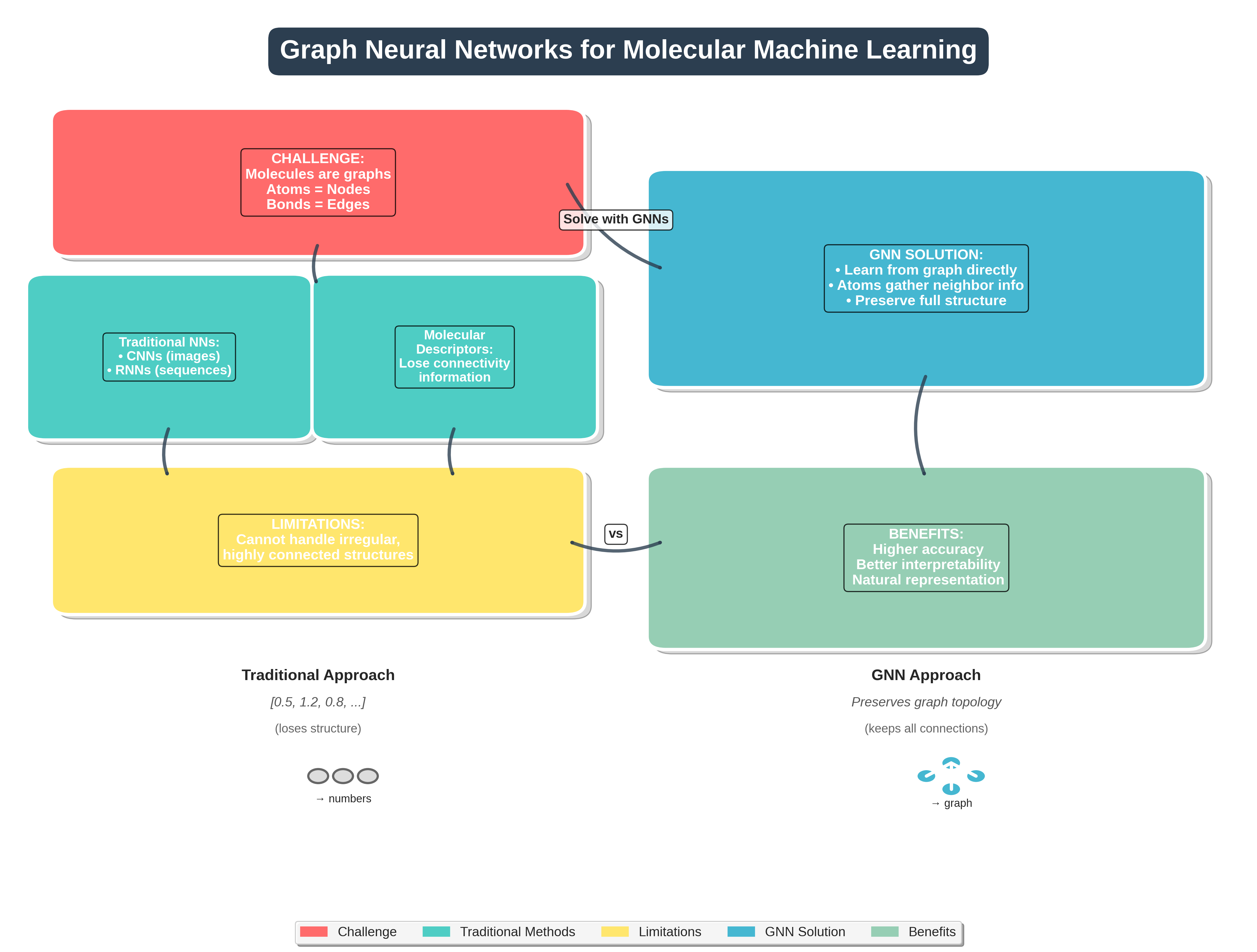 Comparison between traditional neural network approaches and Graph Neural Networks for molecular machine learning. The flowchart illustrates why molecules require graph-based methods and how GNNs preserve structural information that traditional methods lose.
Before GNNs were introduced, chemists used what are known as molecular descriptors. These are numerical features based on molecular structure, such as how many functional groups a molecule has or how its atoms are arranged in space. These descriptors were used as input for machine learning models. However, they often lose important information about the exact way atoms are connected. This loss of detail limits how well the models can predict molecular behavior.
GNNs solve this problem by learning directly from the molecular graph. Instead of relying on handcrafted features, GNNs use the structure itself to learn what matters. Each atom gathers information from its neighbors in the graph, which helps the model understand the molecule as a whole. This approach leads to more accurate predictions and also makes the results easier to interpret.
In short, GNNs allow researchers to build models that reflect the true structure of molecules. They avoid the limitations of older methods by directly using the connections between atoms, offering a more natural and powerful way to predict molecular properties.
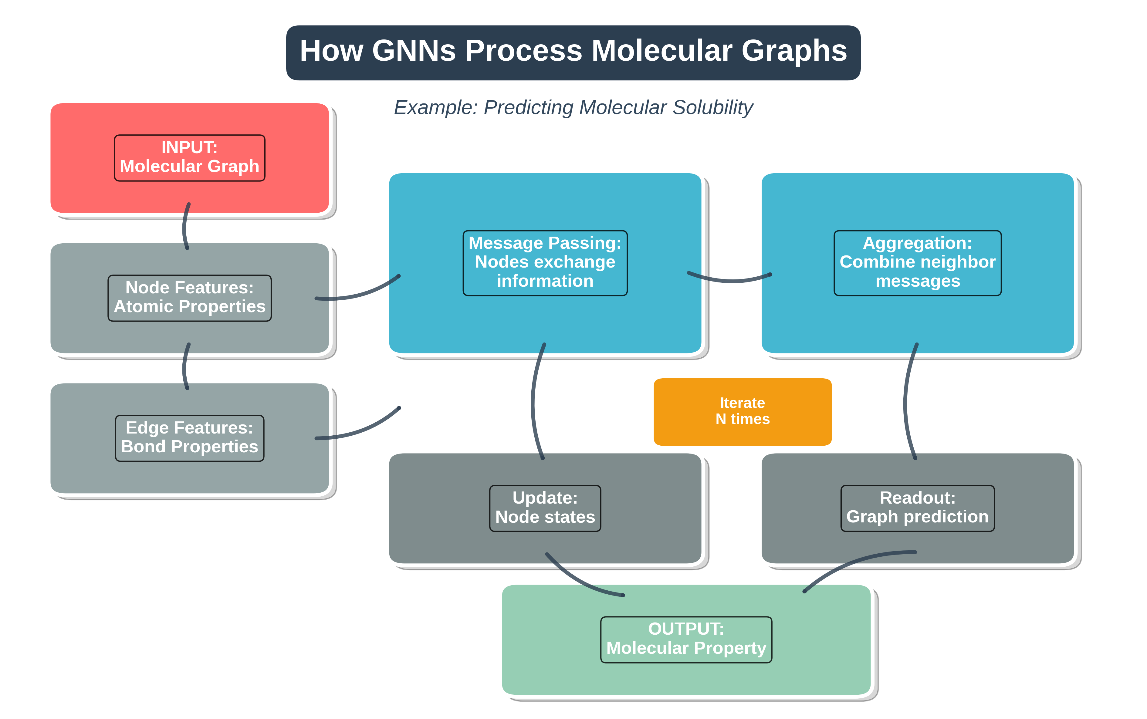 Step-by-step visualization of how Graph Neural Networks process molecular graphs. The pipeline shows the flow from input molecular graph through message passing and aggregation to final property prediction.
3.3.1 What Are Graph Neural Networks?
Completed and Compiled Code: Click Here
Why Are Molecules Naturally Graphs?
Let’s start with the most fundamental question: Why do we say molecules are graphs?
Imagine a water molecule (H₂O). If you’ve taken chemistry, you know it looks like this:
H - O - H
This is already a graph! Let’s break it down:
- Nodes (vertices): The atoms - one oxygen (O) and two hydrogens (H)
- Edges (connections): The chemical bonds - two O-H bonds
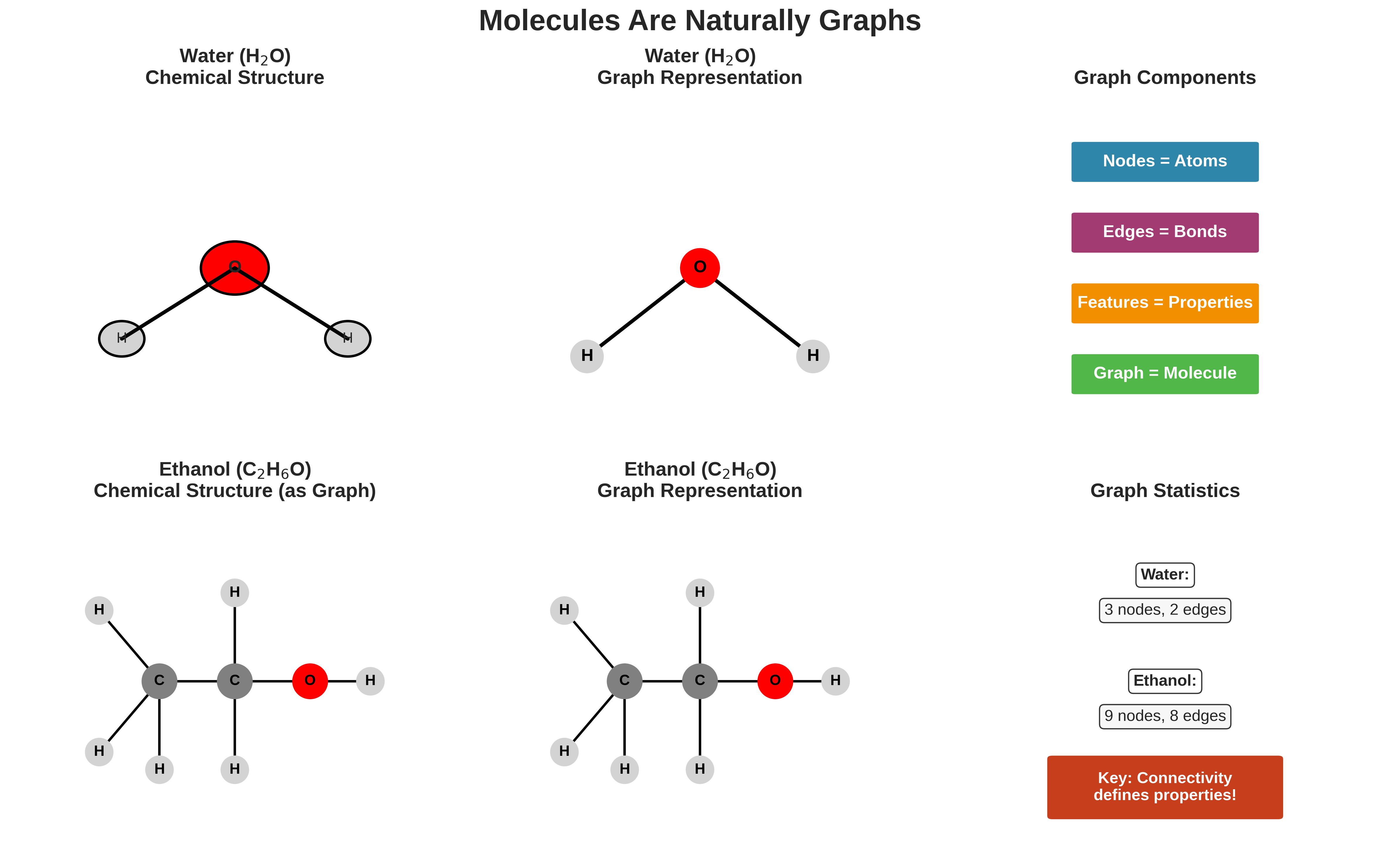 Visualization showing how molecules naturally form graph structures. Water (H₂O) and ethanol (C₂H₆O) are shown in both chemical notation and graph representation, demonstrating that atoms are nodes and bonds are edges.
Now consider a slightly more complex molecule - ethanol (drinking alcohol):
    H H
    | |
H - C-C - O - H
    | |
    H H
Again, we have a graph:
- 9 nodes: 2 carbons, 1 oxygen, 6 hydrogens
- 8 edges: All the chemical bonds connecting these atoms
Here’s the key insight: A molecule’s properties depend heavily on how its atoms are connected. Water dissolves salt because its bent O-H-O structure creates a polar molecule. Diamond is hard while graphite is soft - both are pure carbon, but connected differently!
The Molecular Property Prediction Challenge
Before GNNs, how did computers predict molecular properties like solubility, toxicity, or drug effectiveness? Scientists would calculate numerical “descriptors” - features like:
- Molecular weight (sum of all atom weights)
- Number of oxygen atoms
- Number of rotatable bonds
- Surface area
But this approach has a fundamental flaw. Consider these two molecules:
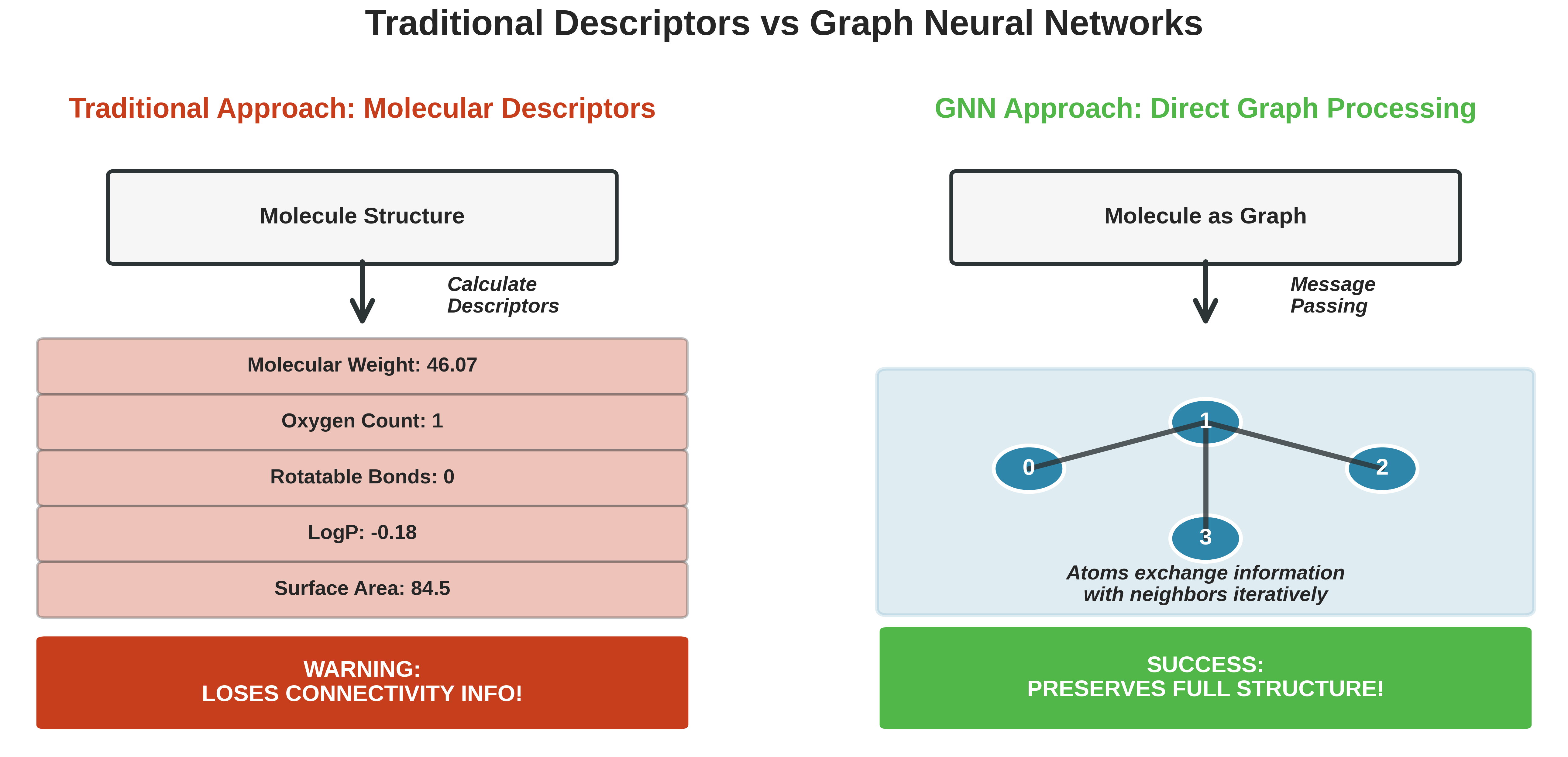 Comparison between traditional molecular descriptors and Graph Neural Networks. Traditional methods lose connectivity information by converting molecules into numerical features, while GNNs preserve the full molecular structure through direct graph processing.
Molecule A:  H-O-C-C-C-C-O-H     (linear structure)
Molecule B:  H-O-C-C-O-H         (branched structure)
                 |
                 C-C
Traditional descriptors might count:
- Both have 2 oxygens ✓
- Both have similar molecular weights ✓
- Both have OH groups ✓
Yet their properties could be vastly different! The traditional approach loses the connectivity information - it treats molecules as “bags of atoms” rather than structured entities.
Enter Graph Neural Networks
GNNs solve this problem elegantly. They process molecules as they truly are - graphs where:
| Graph Component | Chemistry Equivalent | Example in Ethanol |
|---|---|---|
| Node | Atom | C, C, O, H, H, H, H, H, H |
| Edge | Chemical bond | C-C, C-O, C-H bonds |
| Node features | Atomic properties | Carbon has 4 bonds, Oxygen has 2 |
| Edge features | Bond properties | Single bond, double bond |
| Graph | Complete molecule | The entire ethanol structure |
How GNNs Learn from Molecular Graphs
The magic of GNNs lies in message passing - atoms “talk” to their neighbors through bonds. Let’s see how this works step by step:
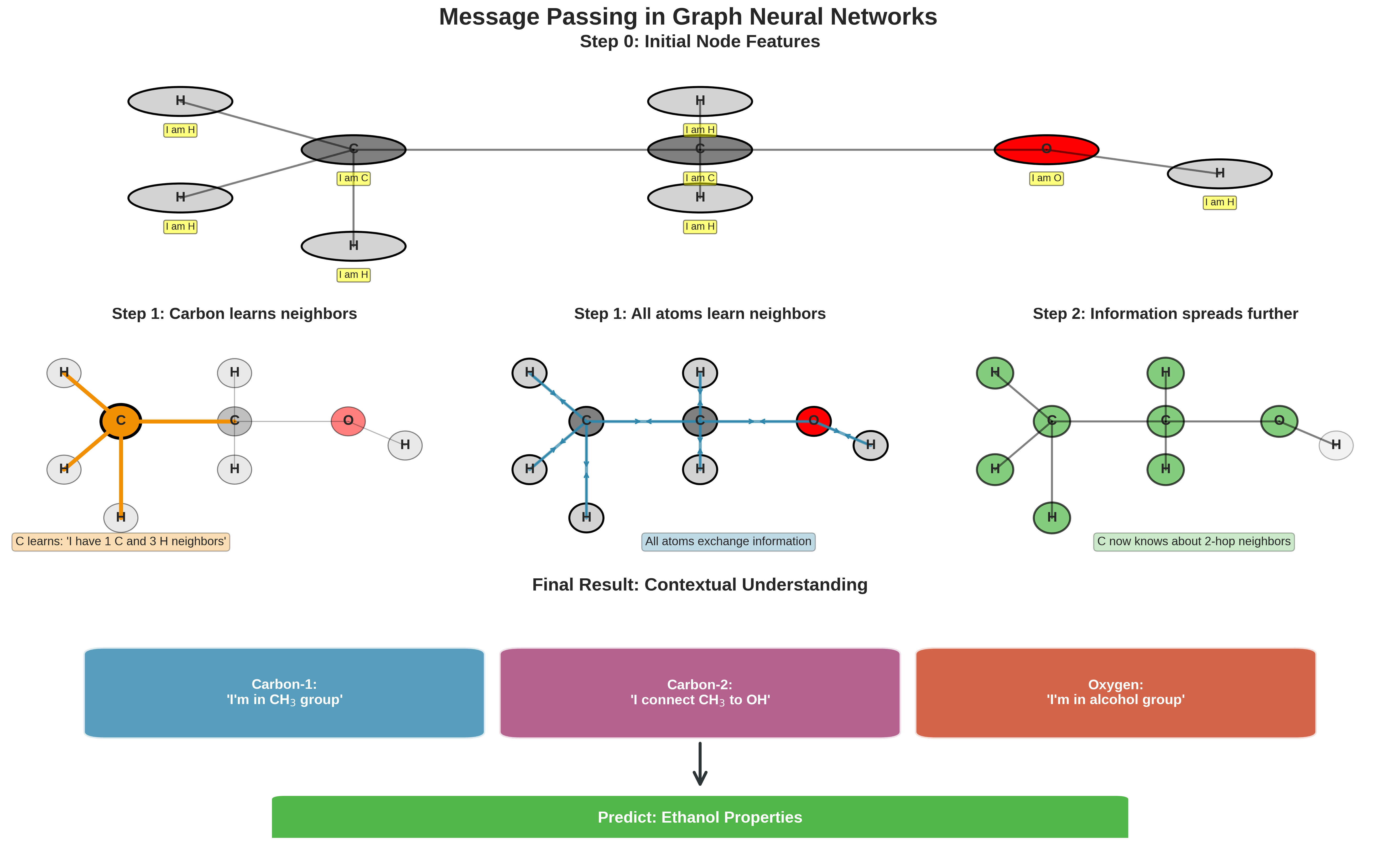 Step-by-step visualization of the message passing mechanism in GNNs. The figure shows how information propagates through the molecular graph over multiple iterations, allowing each atom to understand its role within the larger molecular context.
Step 0: Initial State Each atom starts knowing only about itself:
Carbon-1: "I'm carbon with 4 bonds"
Carbon-2: "I'm carbon with 4 bonds"
Oxygen:   "I'm oxygen with 2 bonds"
Step 1: First Message Pass Atoms share information with neighbors:
Carbon-1: "I'm carbon connected to another carbon and 3 hydrogens"
Carbon-2: "I'm carbon between another carbon and an oxygen"
Oxygen:   "I'm oxygen connected to a carbon and a hydrogen"
Step 2: Second Message Pass Information spreads further:
Carbon-1: "I'm in an ethyl group (CH3CH2-)"
Carbon-2: "I'm the connection point to an OH group"
Oxygen:   "I'm part of an alcohol (-OH) group"
After enough message passing, each atom understands its role in the entire molecular structure!
Why Molecular Property Prediction Matters
Molecular property prediction is at the heart of modern drug discovery and materials science. Consider these real-world applications:
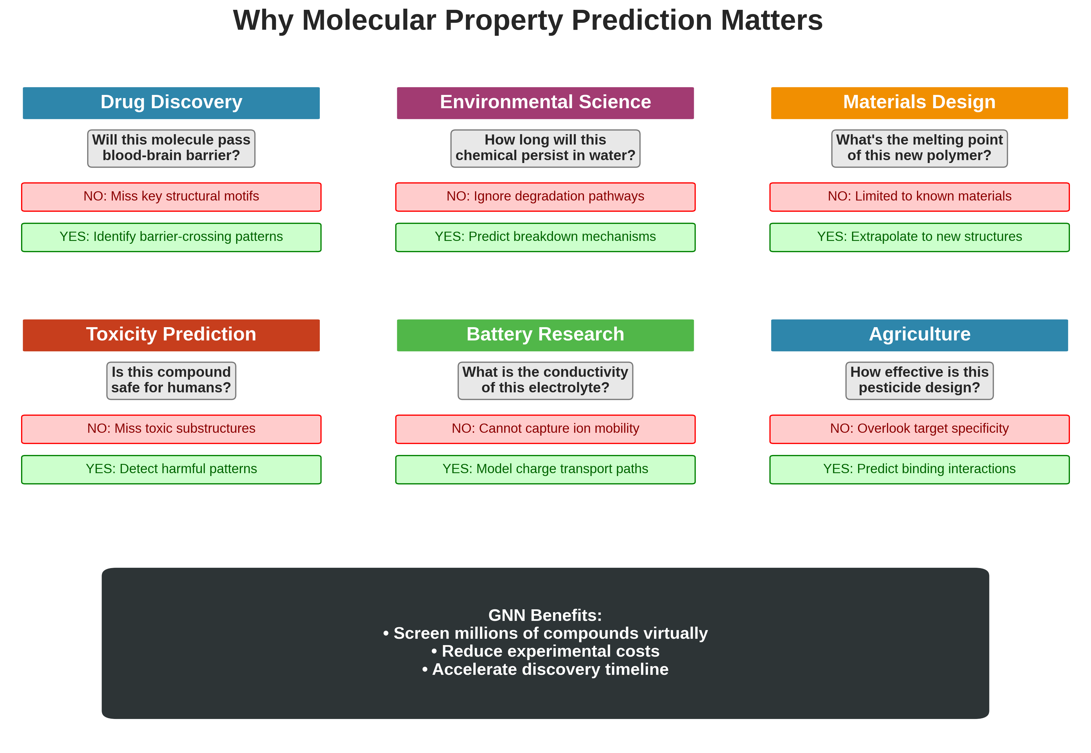 Real-world applications of molecular property prediction using GNNs across six domains: drug discovery, environmental science, materials design, toxicity prediction, battery research, and agriculture.
- Drug Discovery: Will this molecule pass through the blood-brain barrier?
- Environmental Science: How long will this chemical persist in water?
- Materials Design: What’s the melting point of this new polymer?
Traditional experiments to measure these properties are expensive and time-consuming. If we can predict properties from structure alone, we can:
- Screen millions of virtual compounds before synthesizing any
- Identify promising drug candidates faster
- Avoid creating harmful compounds
Representing Molecules as Graphs: A Step-by-Step Guide
Let’s implement a simple example to see how we represent molecules as graphs in code.
We’ll walk step-by-step through a basic molecular graph construction pipeline using RDKit, a popular cheminformatics toolkit in Python. You’ll learn how to load molecules, add hydrogens, inspect atoms and bonds, and prepare graph-based inputs for further learning.
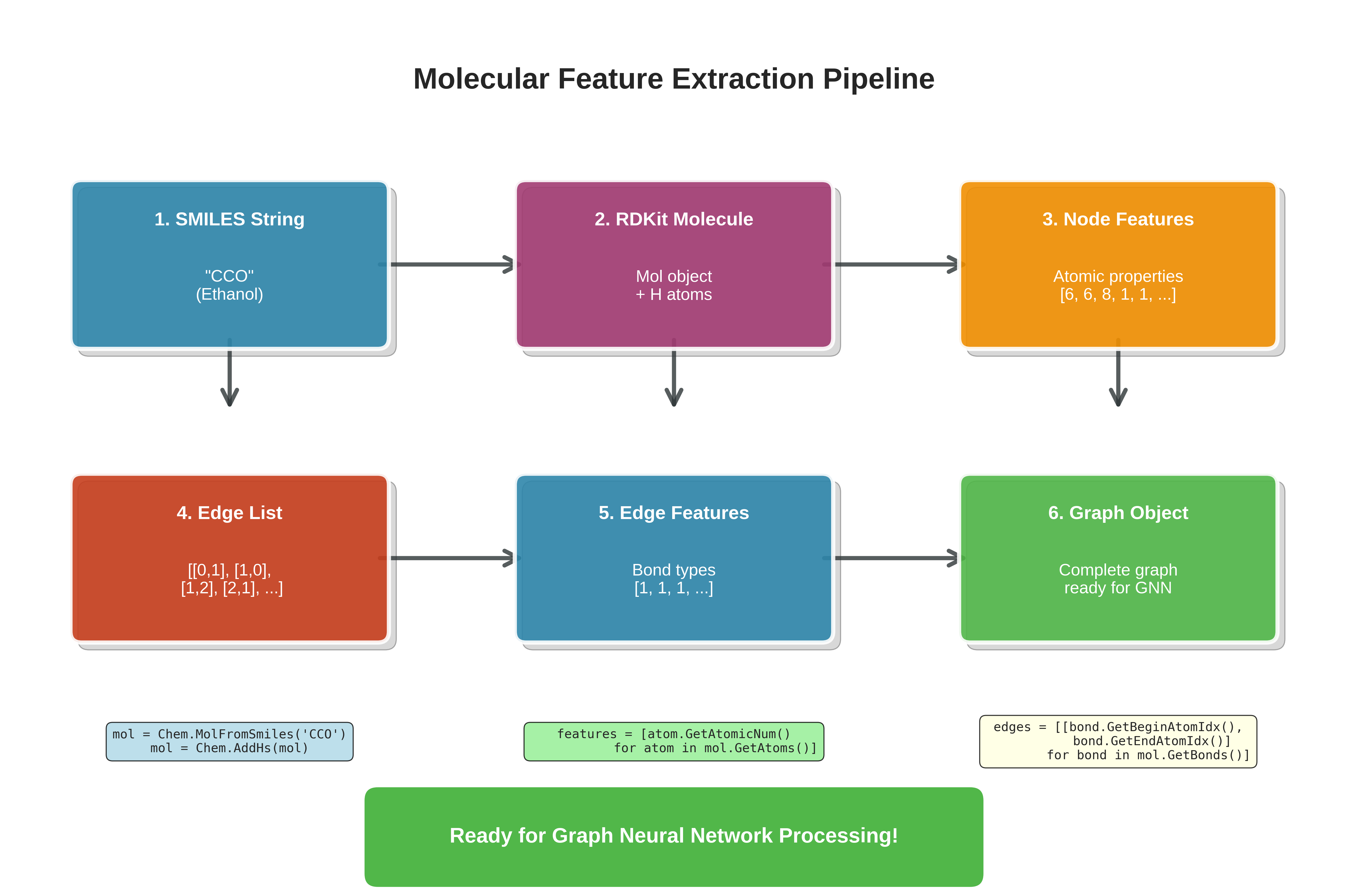 Complete pipeline for converting molecular SMILES strings into graph representations suitable for GNN processing. The workflow shows six stages: from SMILES input through RDKit molecule creation, node/edge feature extraction, to final graph object construction.
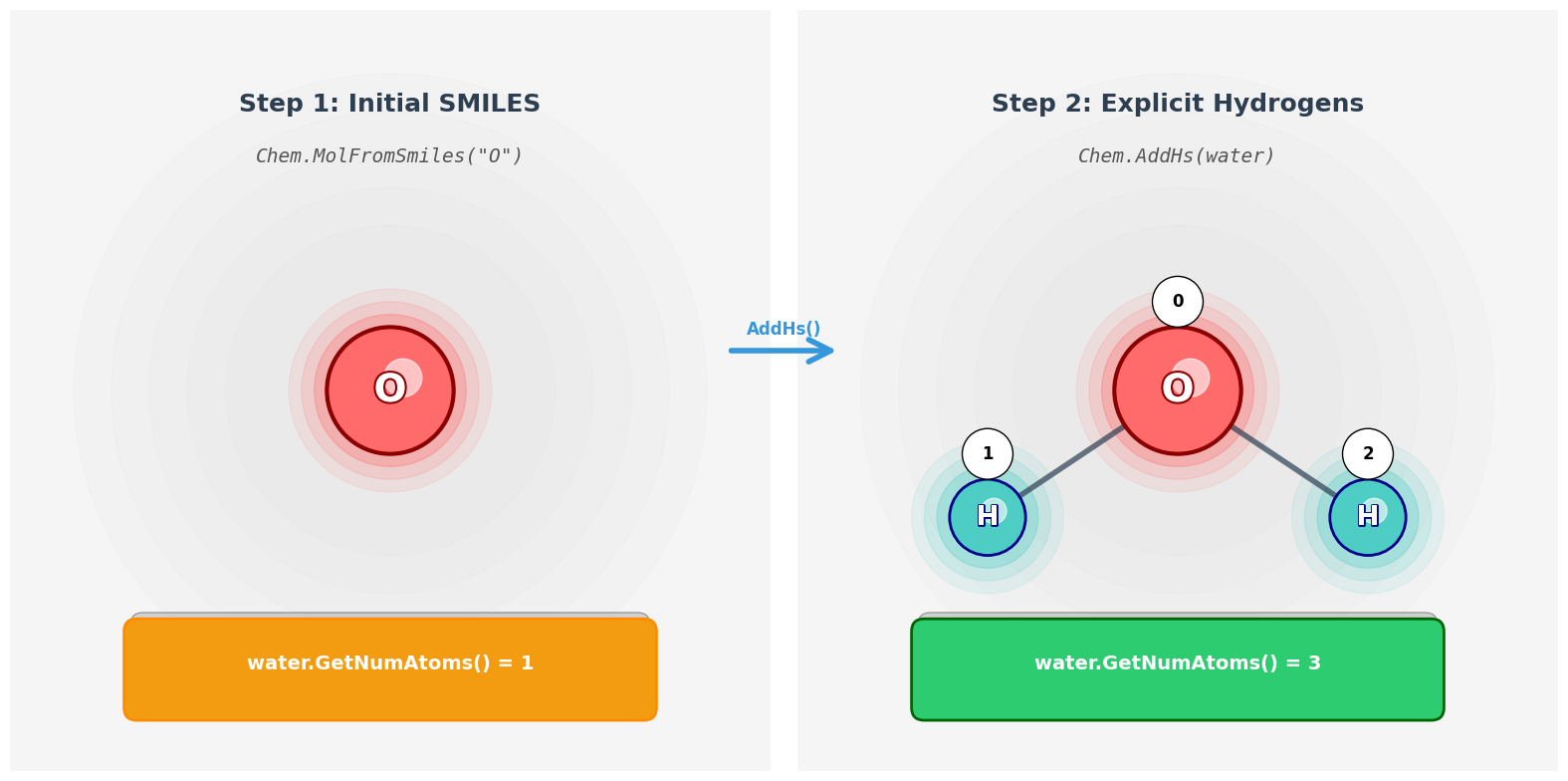
1. Load a molecule and include hydrogen atoms
To start, we need to load a molecule using RDKit. RDKit provides a function Chem.MolFromSmiles() to create a molecule object from a SMILES string (a standard text representation of molecules). However, by default, hydrogen atoms are not included explicitly in the molecule. To use GNNs effectively, we want all atoms explicitly shown, so we also call Chem.AddHs() to add them in.
Let’s break down the functions we’ll use:
-
Chem.MolFromSmiles(smiles_str): Creates anrdkit.Chem.rdchem.Molobject from a SMILES string. This object represents the molecule internally as atoms and bonds. -
mol.GetNumAtoms(): Returns the number of atoms currently present in the molecule object (by default, RDKit does not include H atoms unless you explicitly add them). -
Chem.AddHs(mol): Returns a new molecule object with explicit hydrogen atoms added to the inputmol.
▶ Click to see code: Basic molecule to graph conversion
from rdkit import Chem
import numpy as np

# Step 1: Create a molecule object from the SMILES string for water ("O" means one oxygen atom)
water = Chem.MolFromSmiles("O")

# Count how many atoms are present (will be 1 — only the oxygen)
print(f"Number of atoms: {water.GetNumAtoms()}")  # Output: 1

# Step 2: Add explicit hydrogen atoms
water = Chem.AddHs(water)

# Count again — now we should see 3 atoms (1 O + 2 H)
print(f"Number of atoms with H: {water.GetNumAtoms()}")  # Output: 3
- Initial Atom Count: Initially, the molecule object only includes the oxygen atom, as hydrogen atoms are not explicitly represented by default. Therefore,
GetNumAtoms()returns1. - Adding Hydrogen Atoms: After calling
Chem.AddHs(water), the molecule object is updated to include explicit hydrogen atoms. This is essential for a complete representation of the molecule. - Final Atom Count: The final count of atoms is
3, which includes one oxygen atom and two hydrogen atoms. This accurately reflects the molecular structure of water (H₂O).
By explicitly adding hydrogen atoms, we ensure that the molecular graph representation is comprehensive and suitable for further processing in GNNs.
2. Access the bond structure (graph edges)
Once we have the molecule, we want to know which atoms are connected—this is the basis for constructing a graph. RDKit stores this as a list of Bond objects, which we can retrieve using mol.GetBonds().
Let’s break down the functions used here:
-
mol.GetBonds(): Returns a list of bond objects in the molecule. Each bond connects two atoms. -
bond.GetBeginAtomIdx()andbond.GetEndAtomIdx(): These return the indices (integers) of the two atoms that are connected by the bond. -
mol.GetAtomWithIdx(idx).GetSymbol(): This retrieves the chemical symbol (e.g. “H”, “O”) of the atom at a given index.
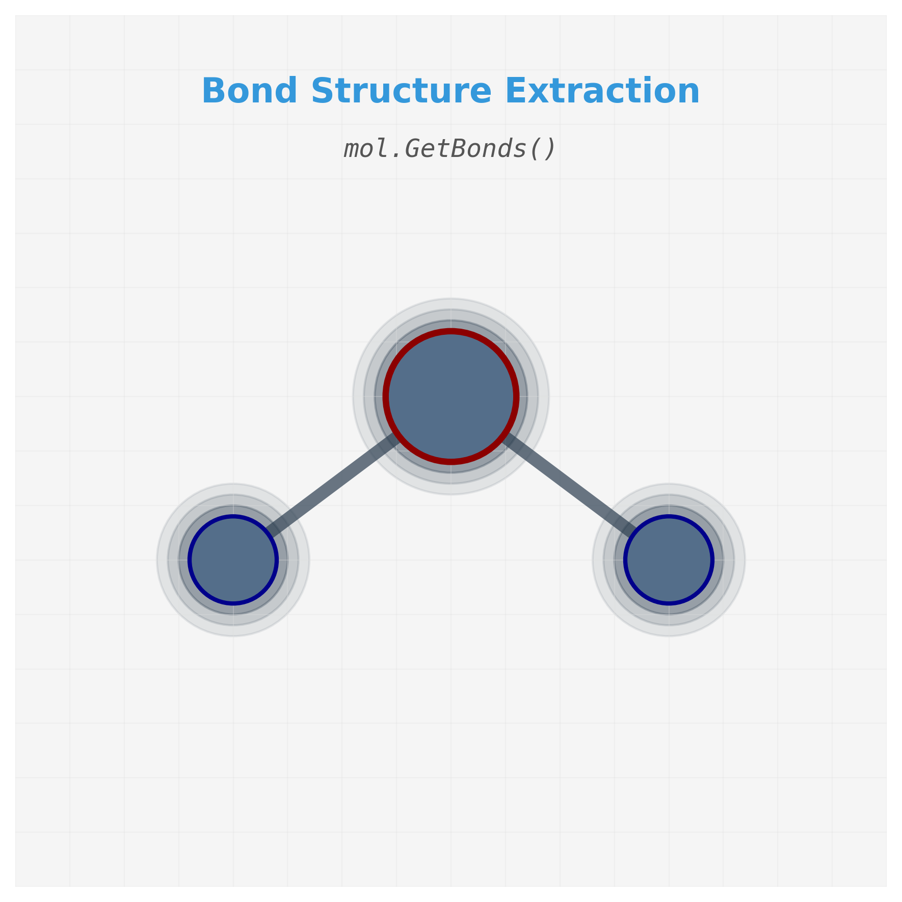 Extracting bond connectivity from RDKit molecule object. Each bond connects two atoms identified by their indices, forming the edges of our molecular graph.
▶ Click to see code: Extracting graph connectivity
# Print all bonds in the molecule in the form: Atom(index) -- Atom(index)
print("Water molecule connections:")
for bond in water.GetBonds():
    atom1_idx = bond.GetBeginAtomIdx()  # e.g., 0
    atom2_idx = bond.GetEndAtomIdx()    # e.g., 1
    atom1 = water.GetAtomWithIdx(atom1_idx).GetSymbol()  # e.g., "O"
    atom2 = water.GetAtomWithIdx(atom2_idx).GetSymbol()  # e.g., "H"
    print(f"  {atom1}({atom1_idx}) -- {atom2}({atom2_idx})")

# Output:
# Water molecule connections:
#   O(0) -- H(1)
#   O(0) -- H(2)
- Bond Retrieval: The
mol.GetBonds()function returns a list of bond objects in the molecule. Each bond object represents a connection between two atoms. - Atom Indices: For each bond,
bond.GetBeginAtomIdx()andbond.GetEndAtomIdx()return the indices of the two atoms connected by the bond. These indices correspond to the positions of the atoms in the molecule object. - Atom Symbols: The
mol.GetAtomWithIdx(idx).GetSymbol()function retrieves the chemical symbol (e.g., “H” for hydrogen, “O” for oxygen) of the atom at a given index. This helps in identifying the types of atoms involved in each bond. - Connectivity Representation: The output shows the connectivity of the water molecule as:
O(0) -- H(1)O(0) -- H(2)
This indicates that the oxygen atom (index 0) is bonded to two hydrogen atoms (indices 1 and 2). This connectivity information is crucial for constructing the graph representation of the molecule, where atoms are nodes and bonds are edges.
3. Extract simple atom-level features
Each atom will become a node in our graph, and we often associate it with a feature vector. To keep things simple, we start with just the atomic number.
Here’s what each function does:
-
atom.GetAtomicNum(): Returns the atomic number (integer) for the element, e.g., 1 for hydrogen, 8 for oxygen. -
mol.GetAtoms(): Returns a generator over allAtomobjects in the molecule. -
atom.GetSymbol(): Returns the chemical symbol (“H”, “O”, etc.), useful for printing/debugging.
 Atom-to-feature mapping. The atomic number provides a simple yet effective initial representation for each node in the molecular graph.
▶ Click to see code: Atom feature extraction
# For each atom, we print its atomic number
def get_atom_features(atom):
    # Atomic number is a simple feature used in many models
    return [atom.GetAtomicNum()]

# Apply to all atoms in the molecule
for i, atom in enumerate(water.GetAtoms()):
    features = get_atom_features(atom)
    symbol = atom.GetSymbol()
    print(f"Atom {i} ({symbol}): features = {features}")

# Output
# Atom 0 (O): features = [8]
# Atom 1 (H): features = [1]
# Atom 2 (H): features = [1]
- Feature Extraction Function:
- The
get_atom_features(atom)function extracts the atomic number of each atom usingatom.GetAtomicNum(). This is a simple yet powerful feature for distinguishing between different elements. - The atomic number is a unique identifier for each element: 1 for hydrogen (H) and 8 for oxygen (O).
- The
- Iterating Over Atoms:
- The
mol.GetAtoms()function returns a generator that iterates over allAtomobjects in the molecule. - For each atom, we retrieve its atomic number and store it as a feature vector (a list containing a single element).
- The
- Output Explanation:
- The output lists each atom in the molecule along with its atomic number:
Atom 0 (O): features = [8]: The oxygen atom (index 0) has an atomic number of 8.Atom 1 (H): features = [1]: The first hydrogen atom (index 1) has an atomic number of 1.Atom 2 (H): features = [1]: The second hydrogen atom (index 2) also has an atomic number of 1.
- The output lists each atom in the molecule along with its atomic number:
- Significance:
- These atomic numbers serve as the initial node features for the molecular graph. In more advanced models, additional features (e.g., degree, hybridization, electronegativity) can be included to capture more complex chemical properties.
- By representing each atom with its atomic number, we provide a basic yet meaningful input for graph neural networks to learn from the structural and chemical properties of the molecule.
In summary, this code demonstrates how to extract simple yet essential features from each atom in a molecule, laying the foundation for constructing informative node attributes in molecular graphs.
4. Build the undirected edge list
Now we extract the list of bonds as pairs of indices. Since GNNs typically use undirected graphs, we store each bond in both directions (i → j and j → i).
Functions involved:
bond.GetBeginAtomIdx(),bond.GetEndAtomIdx()(as above)- We simply collect
[i, j]and[j, i]into a list of edges.
 Building an undirected edge list from molecular bonds. Each bond generates two directed edges (i→j and j→i) to ensure bidirectional message passing in the GNN.The complete edge list for water molecule. Bidirectional edges enable information flow in both directions during GNN message passing.
▶ Click to see code: Edge extraction
def get_edge_list(mol):
    edges = []
    for bond in mol.GetBonds():
        i = bond.GetBeginAtomIdx()
        j = bond.GetEndAtomIdx()
        edges.append([i, j])
        edges.append([j, i])  # undirected graph: both directions
    return edges

# Run on water molecule
water_edges = get_edge_list(water)
print("Water edges:", water_edges)

# Output
# Water edges: [[0, 1], [1, 0], [0, 2], [2, 0]]
- Function Definition:
get_edge_list(mol): This function takes an RDKit molecule object (mol) as input and returns a list of edges representing the connectivity between atoms.
- Edge Extraction:
mol.GetBonds(): This method retrieves a list of bond objects from the molecule. Each bond object represents a connection between two atoms.- For each bond,
bond.GetBeginAtomIdx()andbond.GetEndAtomIdx()are used to get the indices of the two atoms connected by the bond. These indices are integers that uniquely identify atoms within the molecule. - The edge list is constructed by appending both
[i, j]and[j, i]to theedgeslist. This ensures that the graph is undirected, which is essential for GNNs. In an undirected graph, the relationship between nodes is bidirectional, meaning that if atomiis connected to atomj, then atomjis also connected to atomi.
- Output:
- The function returns the complete edge list, which includes all pairs of connected atoms in both directions.
- For the water molecule (H₂O), the output is:
Water edges: [[0, 1], [1, 0], [0, 2], [2, 0]][0, 1]and[1, 0]: These pairs represent the bond between the oxygen atom (index 0) and the first hydrogen atom (index 1).[0, 2]and[2, 0]: These pairs represent the bond between the oxygen atom (index 0) and the second hydrogen atom (index 2).
Each pair represents one connection (bond) between atoms. Including both directions ensures that during message passing, information can flow freely from each node to all its neighbors.
 Using RDKit, we can get the chemical structures and corresponding graph statistics for common molecules (water, ethanol, benzene, and aspirin). Each molecule is shown with its 2D structure alongside graph metrics including node count, edge count, and atom type distribution.
Summary: The Power of Molecular Graphs
Let’s recap what we’ve learned:
- Molecules are naturally graphs - atoms are nodes, bonds are edges
- Traditional methods lose structural information - they treat molecules as bags of features
- GNNs preserve molecular structure - they process the actual connectivity
- Message passing allows context learning - atoms learn from their chemical environment
- Property prediction becomes structure learning - the model learns which structural patterns lead to which properties
In the next section, we’ll dive deep into how message passing actually works, building our understanding step by step until we can implement a full molecular property predictor.
3.3.2 Message Passing and Graph Convolutions
Completed and Compiled Code: Click Here
At the core of a Graph Neural Network (GNN) is the idea of message passing. The goal is to simulate an important phenomenon in chemistry: how electronic effects propagate through molecular structures via chemical bonds. This is something that happens in real molecules, and GNNs try to mimic it through mathematical and computational means.
Let’s first look at a chemistry example. When a fluorine atom is added to a molecule, its high electronegativity doesn’t just affect the atom it is directly bonded to. It causes that carbon atom to become slightly positive, which in turn affects its other bonds, and so on. The effect ripples outward through the structure.
This is exactly the kind of structural propagation that message passing in GNNs is designed to model.
 Comparison of electronic effects propagation in real molecules (left) versus GNN simulation (right). The fluorine atom’s electronegativity creates a ripple effect through the carbon chain, which GNNs capture through iterative message passing.
The structure of message passing: what happens at each GNN layer?
Even though the idea sounds intuitive, we need a well-defined set of mathematical steps for the computer to execute. In a GNN, each layer usually follows three standard steps.
 The three standard steps of message passing in GNNs: (1) Message Construction - neighbors create messages based on their features and edge properties, (2) Message Aggregation - all incoming messages are combined using sum, mean, or attention, (3) State Update - nodes combine their current state with aggregated messages to produce new representations.
Step 1: Message Construction
For every node $i$, we consider all its neighbors $j$ and create a message $m_{ij}$ to describe what information node $j$ wants to send to node $i$.
This message often includes:
- Information about node $j$ itself
- Information about the bond between $i$ and $j$ (e.g., single, double, aromatic)
Importantly, we don’t just pass raw features. Instead, we use learnable functions (like neural networks) to transform the input into something more meaningful for the task.
Step 2: Message Aggregation
Once node $i$ receives messages from all neighbors, it aggregates them into a single combined message $m_i$.
The simplest aggregation method is to sum all incoming messages:
\[m_i = \sum_{j \in N(i)} m_{ij}\]Here, $N(i)$ is the set of all neighbors of node $i$. This step is like saying: “I listen to all my neighbors and combine what they told me.”
However, in real chemistry, not all neighbors are equally important:
- A double bond may influence differently than a single bond
- An oxygen atom might carry more weight than a hydrogen atom
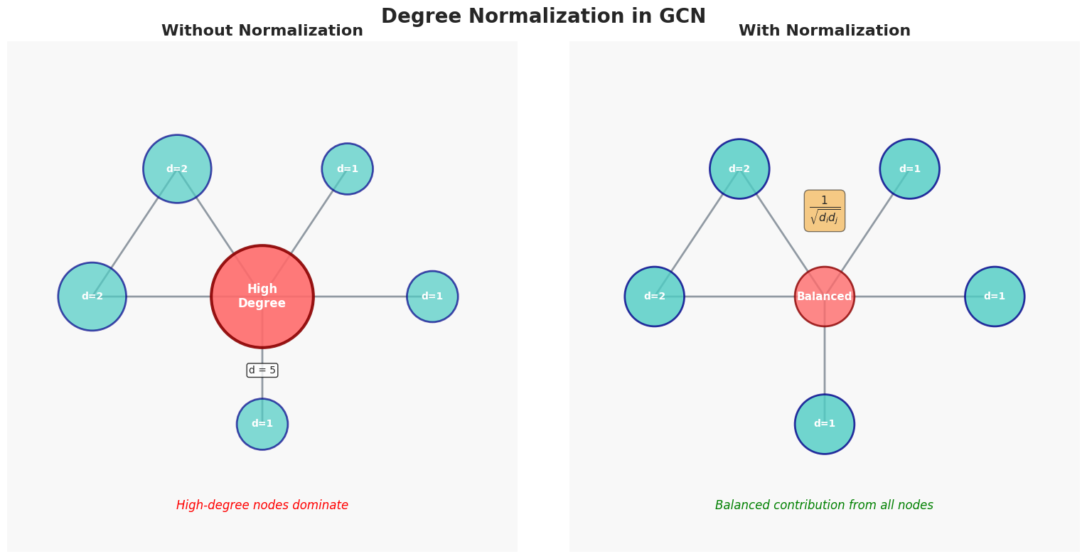
That’s why advanced GNNs often use weighted aggregation or attention mechanisms to adjust how each neighbor contributes.
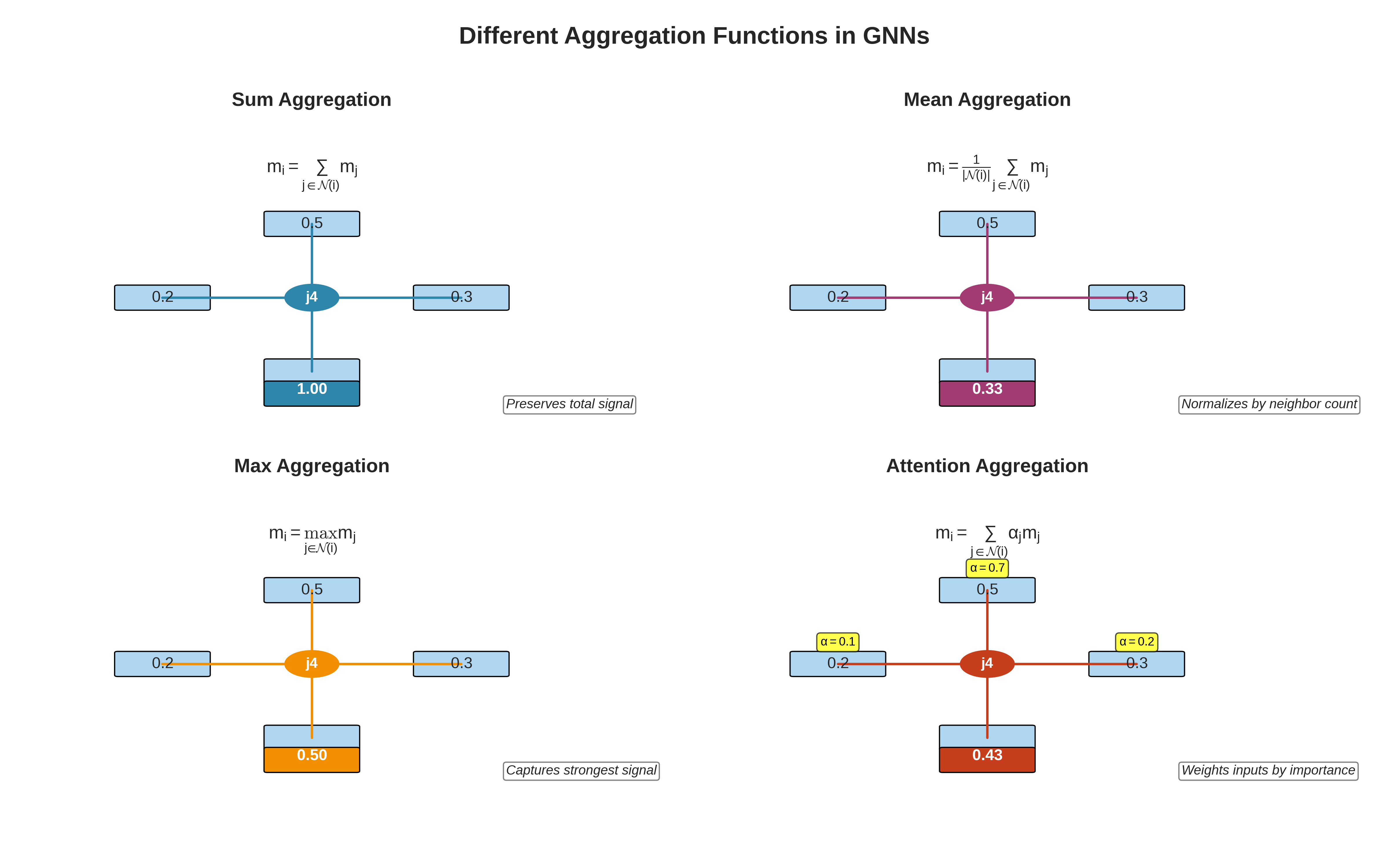 Different aggregation functions in GNNs. Sum preserves total signal strength, Mean normalizes by node degree, Max captures the strongest signal, and Attention weights messages by learned importance scores.
Step 3: State Update
Finally, node $i$ uses two inputs:
- Its current feature vector $h_i^{(t)}$
- The aggregated message $m_i$
These are combined to produce an updated node representation for the next layer:
\[h_i^{(t+1)} = \text{Update}(h_i^{(t)}, m_i)\]This update is usually implemented with a small neural network, such as a multilayer perceptron (MLP). It learns how to combine a node’s old information with the new input from its neighbors to produce something more useful.
In summary, at each GNN layer, every atom (node) listens to its neighbors and updates its understanding of the molecule. After several layers of message passing, each node’s embedding captures not just its local features, but also the broader context of the molecular structure.
Graph Convolutions: Making It Concrete
The term “graph convolution” comes from analogy with Convolutional Neural Networks (CNNs) in computer vision. In CNNs, filters slide over local neighborhoods of pixels. In GNNs, we also aggregate information from “neighbors”, but now neighbors are defined by molecular or structural connectivity, not spatial proximity.
In Graph Convolutional Networks (GCNs), message passing is defined by this formula for at each layer:
\[h_i^{(t+1)} = \sigma \left( \sum_{j \in \mathcal{N}(i) \cup \{i\}} \frac{1}{\sqrt{d_i d_j}} W h_j^{(t)} \right)\]- $h_i^{(t)}$: Feature of node $i$ at layer $t$
- $W$: Learnable weight matrix
- $d_i$: Degree (number of neighbors) of node $i$
- $\sigma$: Activation function (e.g. ReLU)
This formula averages and transforms neighbor features while normalizing based on node degrees.
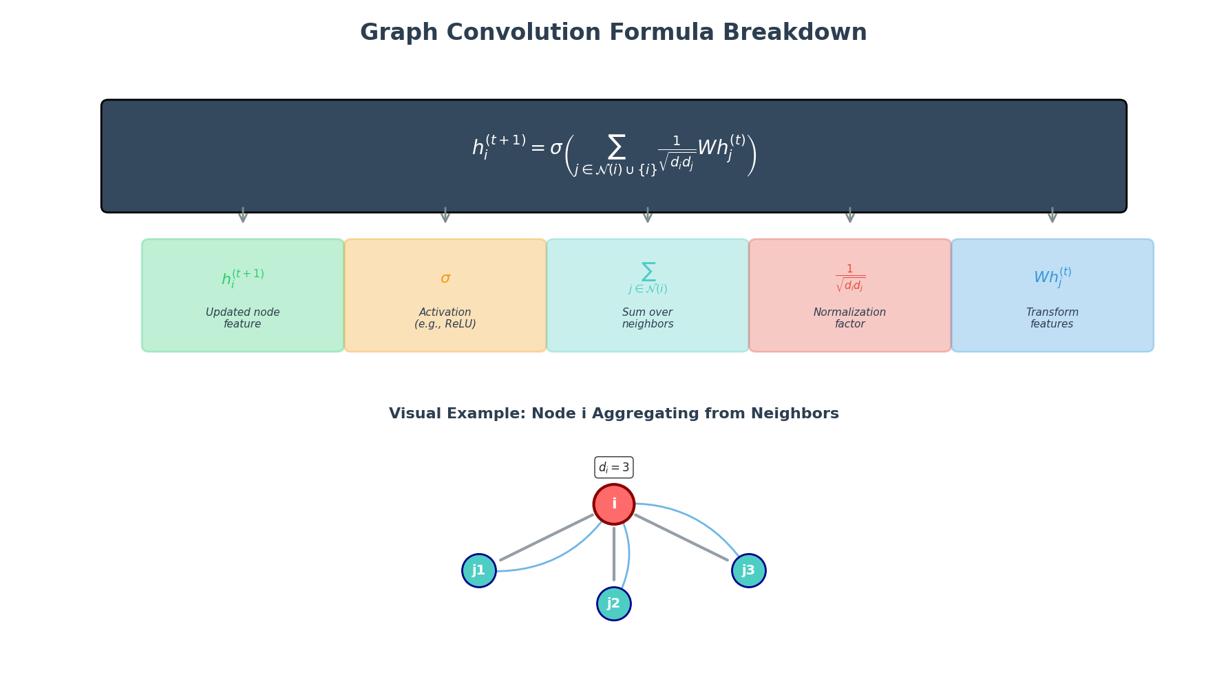
According to the formula, GCN message passing follows 4 steps at each layer:
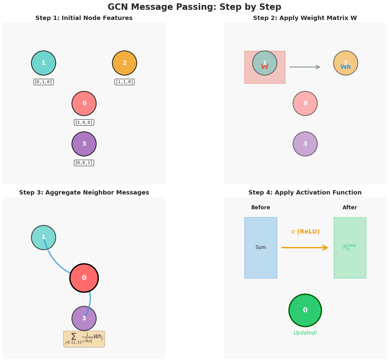
To execute it in Python, we use PyTorch Geometric (PyG). In PyTorch Geometric (PyG), the most basic GNN implementation is GCNConv. Let’s go through each part of the code.
PyTorch Geometric Components
| Component | Purpose |
|---|---|
torch.tensor(...) |
Creates dense tensors (like NumPy arrays) for node features or edge indices. |
x |
Node feature matrix. Shape = [num_nodes, num_node_features] |
edge_index |
Edge list in COO format: [2, num_edges]. First row: source nodes. Second row: target nodes. |
torch_geometric.data.Data |
Creates a graph object holding x, edge_index, and optionally edge/node labels. |
GCNConv(in_channels, out_channels) |
A GCN layer that does: message passing + aggregation + update. |
conv(x, edge_index) |
Applies one layer of graph convolution and returns updated node features. |
Each part of our code works according to this Flowchart:
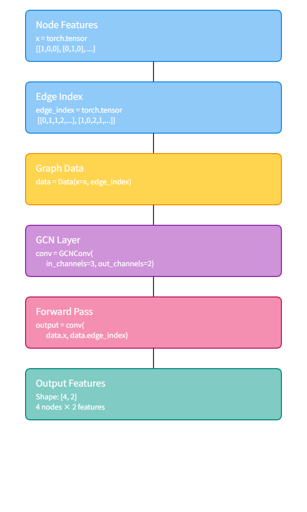
Algorithmic Idea
The flowchart above shows how raw atomic features are transformed by a single GCN (Graph Convolutional Network) layer into learned, structure-aware embeddings. Below, we unpack this transformation step-by-step, both conceptually and computationally.
1. Node Features Each atom is represented by a 3-dimensional one-hot feature vector that encodes its identity. For example:
[1, 0, 0]could represent carbon (C)[0, 1, 0]oxygen (O)[0, 0, 1]nitrogen (N)
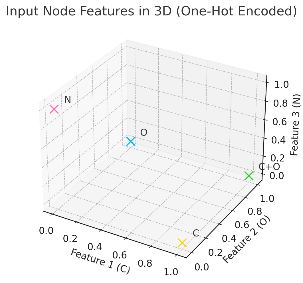
In our toy molecule with 4 atoms, the input node feature matrix has shape [4, 3]: 4 atoms, each with 3 features.
import torch

x = torch.tensor([
    [1, 0, 0],  # Atom 0: C
    [0, 1, 0],  # Atom 1: O
    [1, 1, 0],  # Atom 2: hybrid or multi-type
    [0, 0, 1]   # Atom 3: N
], dtype=torch.float)
This matrix x is the starting point: a basic, structure-free description of the molecule.
2. Edge Index To describe how atoms are bonded, we define the connectivity of the molecular graph using a list of directed edges. Each chemical bond is entered twice to support bidirectional message passing.
The resulting tensor edge_index has shape [2, E], where E is the total number of directed edges. In our case, E = 8.
edge_index = torch.tensor([
    [0, 1, 1, 2, 2, 3, 3, 0],  # Source atoms
    [1, 0, 2, 1, 3, 2, 0, 3]   # Target atoms
], dtype=torch.long)
Here, for example, the edge (0, 1) and (1, 0) encode a bond between atoms 0 and 1.

3. Graph Data
PyTorch Geometric uses a unified object to represent graph-structured data. The node features x and the connectivity edge_index are bundled into a Data object:
from torch_geometric.data import Data

data = Data(x=x, edge_index=edge_index)
At this point:
data.xhas shape [4, 3]data.edge_indexhas shape [2, 8]
This fully defines a small undirected graph of 4 atoms.
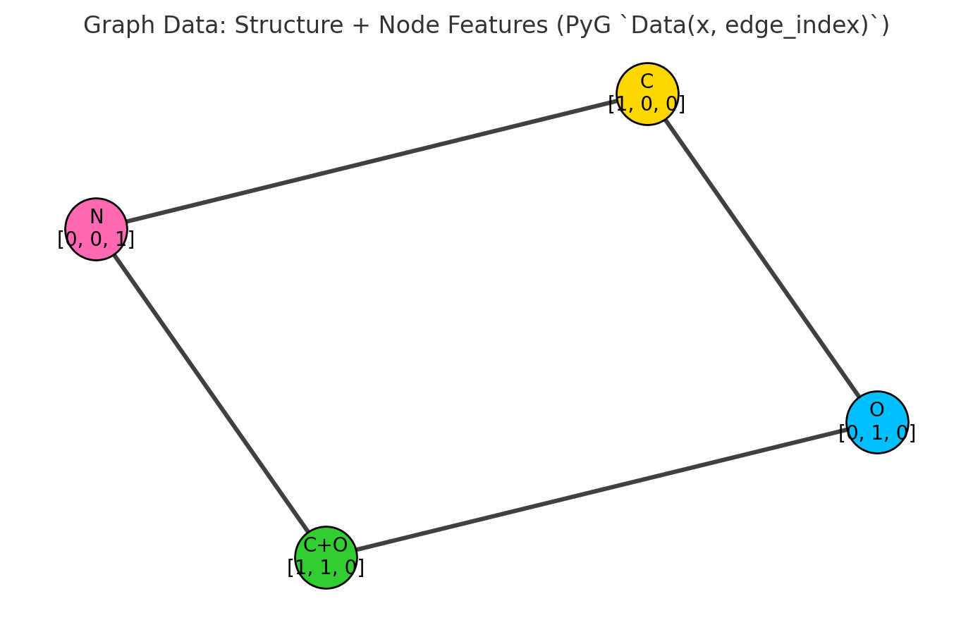
4. GCN Layer We now define a graph convolutional layer that will transform each 3-dimensional atom vector into a 2-dimensional learned embedding.
This is not just a dimensionality reduction step. Rather, it’s a learned transformation:
- It combines each atom’s own features with information from its bonded neighbors
- It applies a shared learnable weight matrix $W \in \mathbb{R}^{3 \times 2}$
- It normalizes contributions based on node degrees
- It applies a non-linear activation function (e.g. ReLU)
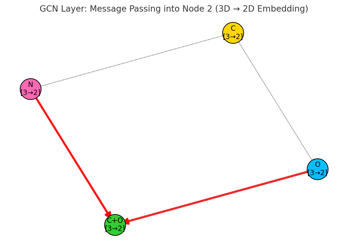
This transformation implements the formula:
\[h_i^{(t+1)} = \sigma \left( \sum_{j \in \mathcal{N}(i) \cup \{i\}} \frac{1}{\sqrt{d_i d_j}} \, W h_j^{(t)} \right)\]Where:
- $h_j^{(t)}$ is the 3-dimensional feature vector of neighbor $j$
- $W$ maps from 3 → 2 dimensions
- $\sigma$ is a nonlinearity (e.g. ReLU)
- The normalization factor $\frac{1}{\sqrt{d_i d_j}}$ accounts for node degrees
The layer is defined as:
from torch_geometric.nn import GCNConv

conv = GCNConv(in_channels=3, out_channels=2)
This means: input is a [4, 3] matrix, and output will be a [4, 2] matrix. Each atom now gets a 2-dimensional embedding.
Why go from 3 to 2 dimensions? We are not blindly compressing the input — rather, we are learning a more compact, expressive representation that fuses both identity and structure. The dimensionality is a design choice: you could use 2, 8, 128… depending on downstream task complexity. In this toy case, 2 is used for visualization and simplicity.
5. Forward Pass We now execute the forward pass of the GCN. Internally, the layer:
- For each atom, gathers features from its neighbors and itself
- Applies the learned transformation and aggregates
- Outputs a new feature vector per atom
output = conv(data.x, data.edge_index)
After this operation:
- Input shape: [4, 3]
- Output shape: [4, 2]
- Each row in the output is a learned embedding vector for an atom
6. Output Features
print("Updated Node Features After Message Passing:")
print(output)
Result
Updated Node Features After Message Passing:
tensor([[ 0.2851, -0.0017],
        [ 0.6568, -0.4519],
        [ 0.6180,  0.1266],
        [ 0.2807, -0.3559]], grad_fn=<AddBackward0>)
Interpretation
Shape: The output has shape [4, 2]:
- 4 rows → 4 atoms
- 2 columns → each atom’s learned embedding
What does each embedding mean?
Each row (e.g. [0.2851, -0.0017]) represents an atom’s updated feature — not just its raw type (C, O, N), but also how it is situated in the molecular graph:
- Who its neighbors are
- What types they are
- How strongly it’s connected (degree)
This embedding is no longer one-hot or fixed — it is learned from data, and will improve with training.
Why is this useful?
You can now:
- Feed these embeddings into another neural network to predict molecular properties
- Use them to classify atom roles (e.g., is this a reaction site?)
- Visualize molecule structure in 2D/3D via t-SNE or PCA
About grad_fn=<AddBackward0>
This line tells you that the output is part of the autograd computation graph in PyTorch. That means it supports backpropagation: gradients will flow back through the GCN layer during training to update $W$.
Variants of Graph Convolutions
Different GNN models define the message passing process differently:
Graph Convolutional Networks (GCNs) Use simple averaging with normalization. Very stable and interpretable. Good for small graphs with clean structure.
GraphSAGE Introduces neighbor sampling, which makes it scalable to large graphs. You can also choose the aggregation function (mean, max, LSTM, etc.).
Graph Attention Networks (GATs) Use attention to assign different weights to different neighbors. This is very helpful in chemistry, where some bonds are more important (e.g. polar bonds).
Message Passing Neural Networks (MPNNs) A general and expressive framework. Can use edge features, which is important in molecules (e.g. bond type, aromaticity). Many SOTA chemistry models (e.g., D-MPNN) are built on this.
 Figure 3.3.10: Comparison of different GNN architectures. GCN uses simple normalized averaging, GraphSAGE samples neighbors for scalability, GAT employs attention mechanisms for weighted aggregation, and MPNN provides a general framework incorporating edge features.
Chemical Intuition Behind Message Passing
To understand how message passing in graph neural networks actually captures chemical effects, let’s walk through a concrete example: the molecule para-nitrophenol, which features two chemically distinct groups — a nitro group (NO₂) and a hydroxyl group (OH) — placed at opposite ends of a benzene ring.
Chemically speaking, this setup forms a classic “push-pull” system: the nitro group is strongly electron-withdrawing, while the hydroxyl group is electron-donating. This dynamic tension in electron distribution plays a key role in determining the molecule’s acidity, reactivity, and overall behavior. The power of message passing lies in its ability to gradually capture this electron flow, layer by layer.
 Figure 3.3.11: Receptive field expansion in GNNs. Each layer increases a node’s awareness by one hop. Starting from self-awareness (Layer 0), nodes progressively integrate information from 1-hop neighbors, 2-hop neighbors, and eventually the entire molecular graph.
GNN Message Passing: Neighborhood Expansion per Layer
- Layer 0: Self (Each atom only knows its own features)
- e.g., O knows it’s oxygen; N knows it’s nitrogen
- Layer 1: 1-hop neighbors (Directly bonded atoms)
- O learns about the carbon it’s attached to
- N in NO₂ learns about its adjacent O atoms
- Layer 2: 2-hop neighbors (Neighbors of neighbors)
- O learns about atoms bonded to its neighboring carbon
- Benzene carbons begin to capture influence from NO₂ and OH
- Layer 3: 3-hop neighborhood (Extended molecular context)
- Carbons across the ring begin to “feel” opposing substituent effects
- Push-pull interactions emerge in representation
- Layer 4+: Global context (Full molecule representation)
- Every atom integrates information from the entire molecule
- Final features encode global electronic and structural effects
Summary
In this section, we explored message passing and graph convolutions, the fundamental mechanisms that enable Graph Neural Networks to learn from molecular structures. The key insight is that GNNs mimic how electronic effects propagate through chemical bonds in real molecules.
The message passing framework follows three standard steps at each layer:
- Message Construction: Nodes create messages for their neighbors using learnable functions
- Message Aggregation: Each node combines incoming messages (via sum, attention, etc.)
- State Update: Nodes update their representations by combining current features with aggregated messages
Through the lens of para-nitrophenol, we saw how this iterative process gradually expands each atom’s “awareness” from local to global context. Starting with only self-knowledge, atoms progressively integrate information from direct neighbors, then second-hop neighbors, until eventually capturing full molecular context including competing electronic effects.
Different GNN architectures (GCN, GraphSAGE, GAT, MPNN) offer various approaches to this process, each with distinct advantages for chemical applications. The choice depends on factors like molecular size, importance of edge features, and computational constraints.
The power of message passing lies in its ability to bridge structure and function. By allowing atoms to “communicate” through bonds, GNNs learn representations that encode not just molecular topology, but also the chemical behaviors that emerge from that structure — acidity, reactivity, electronic distribution, and more. This makes GNNs particularly well-suited for molecular property prediction and drug discovery tasks where understanding chemical context is crucial.
3.3.3 GNNs for Molecular Property Prediction
Completed and Compiled Code: Click Here
Experimental Pipeline Overview
What We’re Building: A Molecular Solubility Predictor
Why Predict Molecular Solubility?
- Drug Discovery: 90% of drug candidates fail due to poor solubility – we need to predict this early!
- Cost Savings: Lab testing costs $1000+/molecule; our model predicts in milliseconds
- Real Impact: Better solubility = better drug absorption = more effective medicines
What you’ll learn: How to turn molecules into graphs and use AI to predict their properties
| Stage | Input | Process | Output |
|---|---|---|---|
| 1. Data Loading | ESOL CSV file | pandas parsing | SMILES + log S values |
| 2. Molecular Encoding | SMILES strings (text) |
RDKit → graph conversion | Node features + edge indices |
| 3. Model Building | Graph structures | 3-layer GCN | Molecular embeddings |
| 4. Training | Batched graphs | Adam optimizer + MSE loss | Trained parameters |
| 5. Prediction | New SMILES | Forward pass | Solubility (log S) |
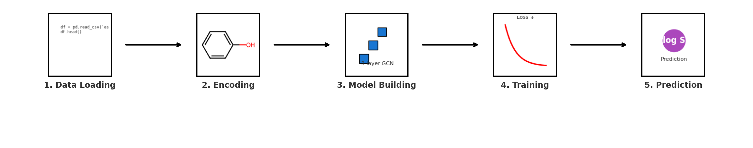
Key Metrics We’ll Track:
- RMSE: Root Mean Squared Error (expect ~1.9 log S)
- R²: Variance explained (expect ~0.22)
- MAE: Mean Absolute Error (expect ~1.6 log S)
Key Terms Explained
| Term | Simple Explanation | Why It Matters |
|---|---|---|
| SMILES | Text code for molecules (like “H₂O” but more detailed) | Computers can’t see molecules, so we use text |
| Node Features | Properties of each atom (e.g. element type, charge) | AI needs numbers to work with |
| Edge Indices | Which atoms are connected by bonds | Structure determines properties |
| GCN | Graph Convolutional Network – AI for graph data | Molecules are naturally graphs! |
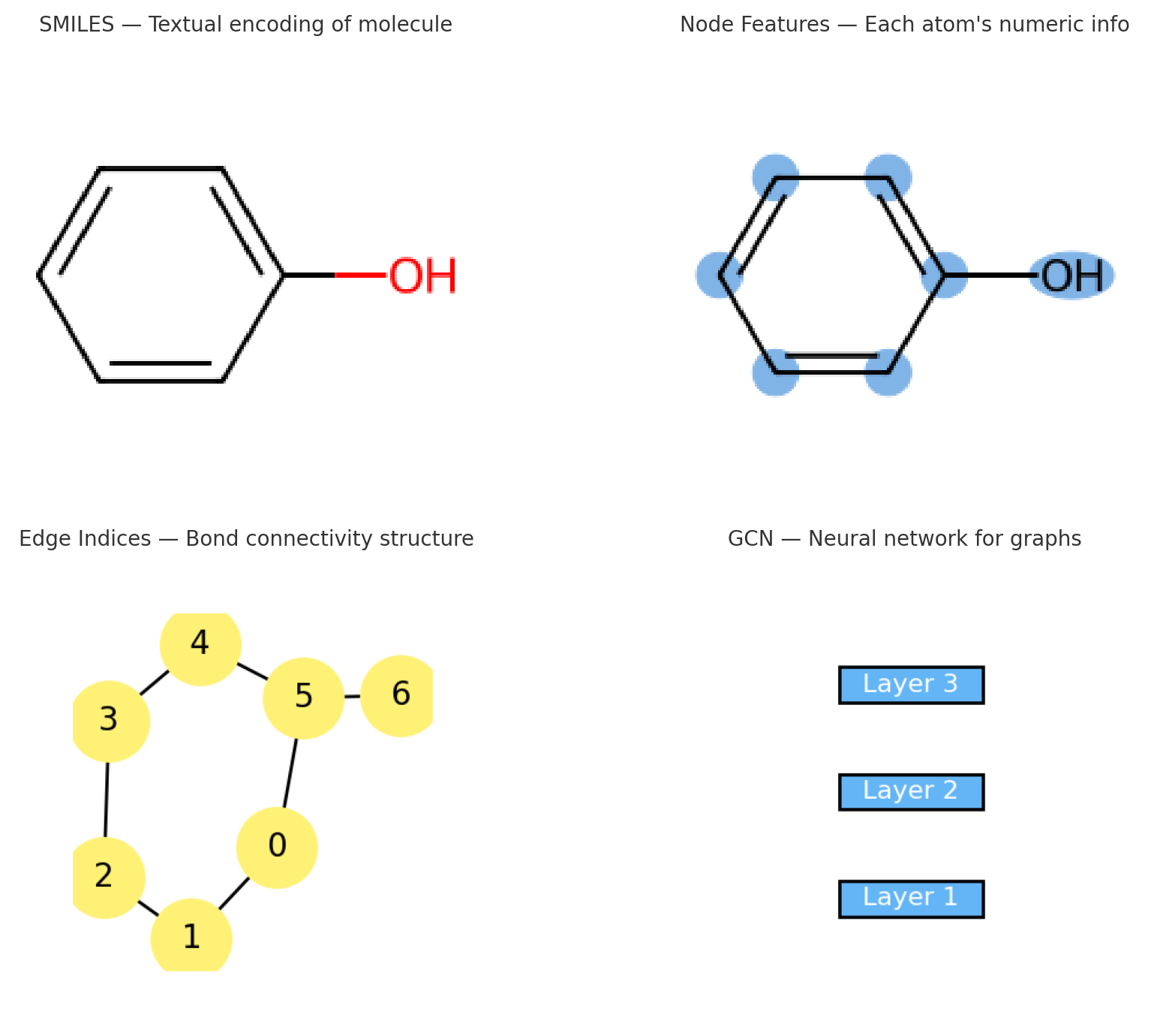
Step 1: Understanding Molecular Solubility as a Graph Learning Problem
The Chemistry Behind Solubility
Why is solubility prediction hard? Solubility emerges from a delicate balance of intermolecular forces:
\[\mathrm{Solubility} \;\propto\; \frac{\text{Solute–Solvent interactions}}{\text{Solute–Solute interactions}}\]What This Formula Really Means:
- Numerator (top): How well the molecule “likes” water
- Denominator (bottom): How much the molecule “likes” itself
- Result: If molecules prefer water over themselves → high solubility!
Example: Sugar dissolves because it forms hydrogen bonds with water better than with other sugar molecules
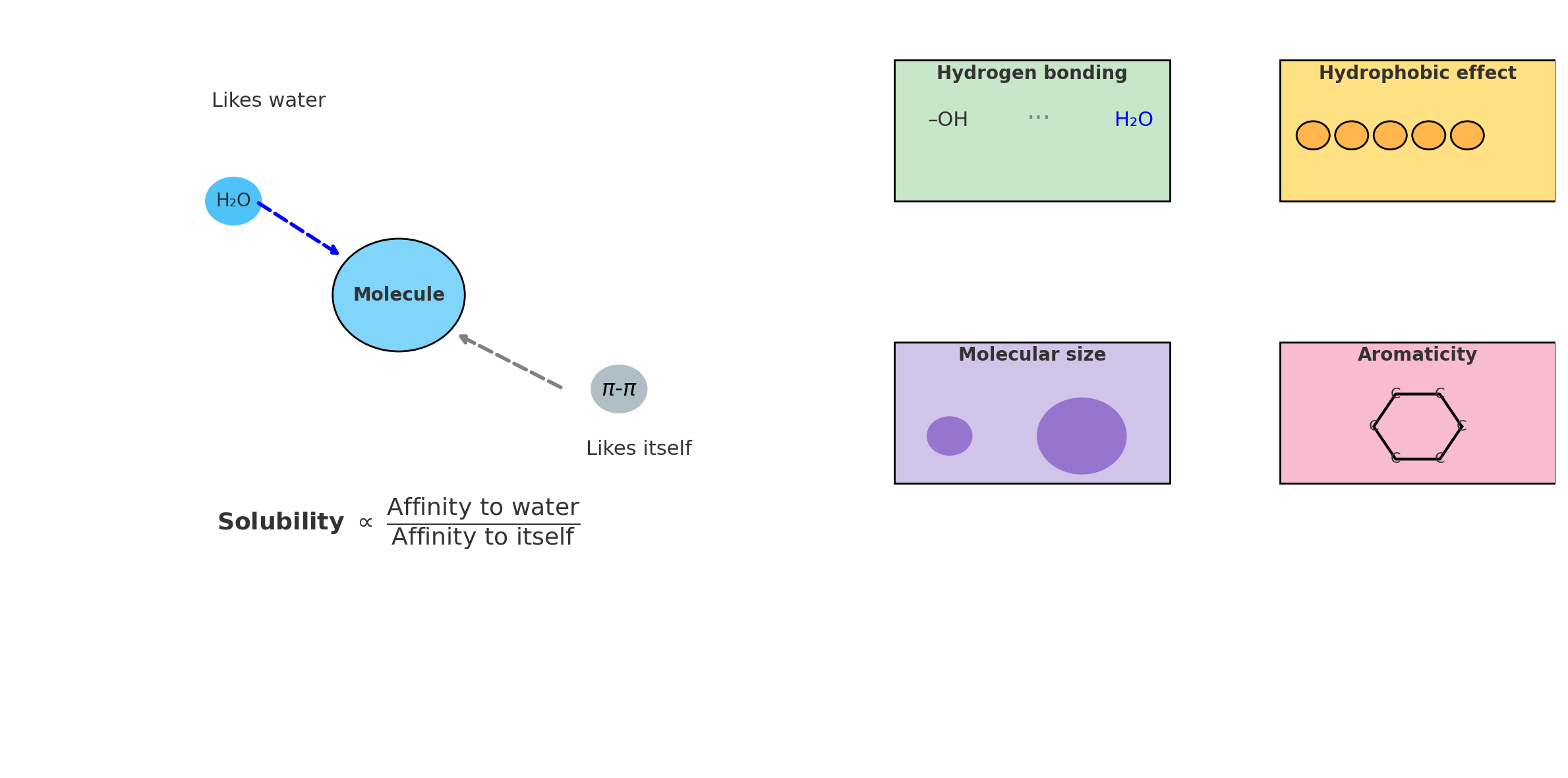
Key factors:
- Hydrogen bonding: –OH, –NH groups increase water solubility
- Hydrophobic effect: Long carbon chains decrease solubility
- Molecular size: Larger molecules → harder to solvate
- Aromaticity: π-systems are hydrophobic
Why Graph Neural Networks?
Traditional machine learning uses fixed-size molecular fingerprints, losing structural information. GNNs preserve the full molecular graph:
Molecule as Graph:
- Nodes: Atoms with features (element, charge, aromaticity)
- Edges: Chemical bonds (single, double, triple, aromatic)
- Message Passing: Atoms “communicate” through bonds
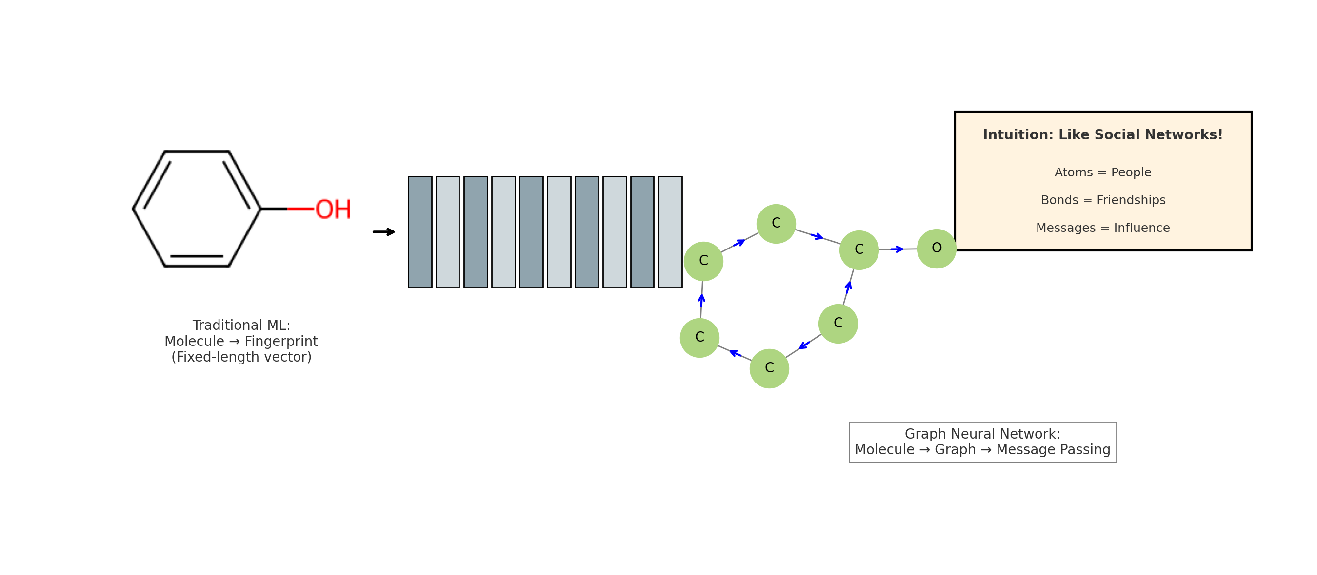
Intuition:
-
Just like social networks!
- People (atoms) have properties (age, interests)
- Friendships (bonds) connect people
- Information spreads through connections
- Your friends influence your behavior!
Step 1.1: Package Imports and Setup
We need several specialized libraries to handle different aspects of the pipeline:
| Step | Library | Purpose | Why We Need It |
|---|---|---|---|
| 1 | PyTorch | Deep Learning Core | Handles neural networks and gradients |
| 2 | PyTorch Geometric | Graph Operations | Special tools for graph neural networks |
| 3 | RDKit | Chemistry Processing | Understands molecules and bonds |
| 4 | NumPy / Pandas | Data Handling | Efficient array and table operations |
| 5 | Scikit-learn | Evaluation Metrics | Measure how good our predictions are |
| Library Import Process | |||
|---|---|---|---|
|
Step 1: Import PyTorch Core torch, nn, F |
Step 2: Import Graph Tools GCNConv, DataLoader |
Step 3: Import Chemistry RDKit Chem module |
Step 4: Import Utilities numpy, pandas, sklearn |
# Deep Learning Framework
import torch
import torch.nn as nn
import torch.nn.functional as F

# Graph Neural Network Operations
from torch_geometric.nn import GCNConv, global_mean_pool
from torch_geometric.data import Data, DataLoader

# Chemistry Toolkit
from rdkit import Chem

# Data Processing & Visualization
import numpy as np
import pandas as pd
import matplotlib.pyplot as plt
import requests
import io
from sklearn.metrics import mean_squared_error, r2_score
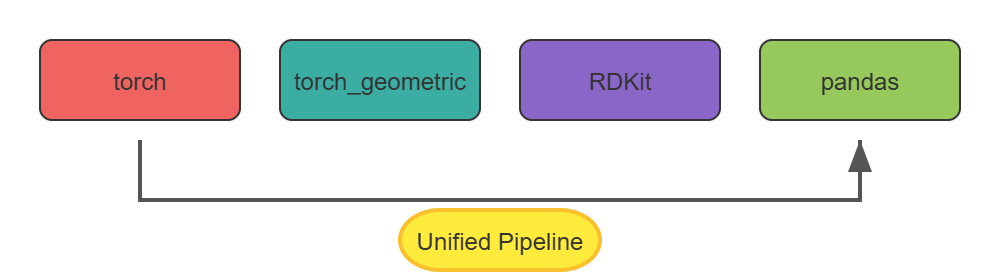
Step 1.2: Feature Extraction
Each atom’s properties influence molecular behavior. We encode 5 key atomic features:
| Feature | Chemical Meaning | Value Range | Why It Affects Solubility |
|---|---|---|---|
| Atomic Number | Element identity (C=6, N=7, O=8) | 1-118 | O, N form H-bonds with water |
| Degree | Number of bonds | 0-4 (typically) | More bonds = less flexible |
| Formal Charge | Electronic state | -2 to +2 | Charged = water-loving |
| Aromaticity | In aromatic ring? | 0 or 1 | Aromatic = water-fearing |
| H Count | Hydrogen bonding potential | 0-4 | More H = more H-bonds |
Implementation: The get_atom_features function extracts these properties from RDKit atom objects:
def get_atom_features(atom):
    """
    Extract numerical features from RDKit atom object.
    These features capture the chemical environment of each atom.

    Think of this as creating an "ID card" for each atom with 5 key facts!
    """
    return [
        atom.GetAtomicNum(),        # What element? (C=6, N=7, O=8, etc.)
        atom.GetDegree(),           # How many bonds? (connectivity)
        atom.GetFormalCharge(),     # Is it charged? (+1, 0, -1, etc.)
        int(atom.GetIsAromatic()),  # In benzene-like ring? (0=no, 1=yes)
        atom.GetTotalNumHs()        # How many hydrogens attached?
    ]
| Atom Feature Extraction Process | ||
|---|---|---|
|
Input: RDKit Atom Object Contains all chemical info |
→ Extract 5 Features → 1. Element type 2. Bond count 3. Charge state 4. Aromaticity 5. H-bond potential |
Output: List of 5 numbers [8, 2, 0, 0, 0] for oxygen |
Why These 5 Features?
- Atomic Number: Oxygen atoms love water, carbon atoms don’t
- Degree (Connectivity): Highly connected atoms are “buried” in the molecule
- Formal Charge: Charged molecules dissolve like salt in water
- Aromaticity: Benzene rings are oily, not watery
- H Count: More hydrogens = more hydrogen bonding with water
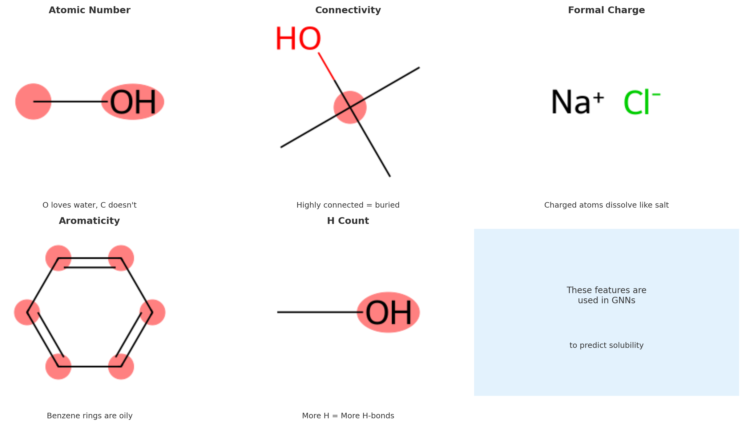
Step 1.3: Bond Connectivity Extraction
Chemical bonds are bidirectional - electrons are shared between atoms. We need to represent this bidirectionality:
| Bond Extraction Process | |||
|---|---|---|---|
|
Step 1: Loop through bonds mol.GetBonds() |
Step 2: Get atom indices i = start, j = end |
Step 3: Create bidirectional [i→j] and [j→i] |
Result: Edge list [[0,1], [1,0], ...] |
def get_bond_connections(mol):
    """
    Convert molecular bonds to directed edges.
    Bidirectional to allow information flow in both directions.

    Why bidirectional? In real molecules, electrons flow both ways!
    """
    edges = []
    for bond in mol.GetBonds():
        i = bond.GetBeginAtomIdx()
        j = bond.GetEndAtomIdx()
        edges.extend([[i, j], [j, i]])  # Add both directions
    return edges
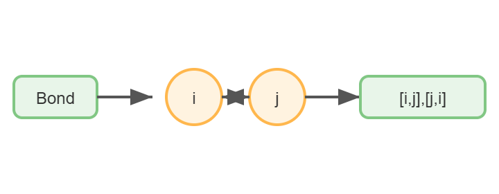
Step 2: Loading and Exploring the ESOL Dataset
Step 2.1: Dataset Overview
Why ESOL? The ESOL (Estimated SOLubility) dataset is a gold standard because:
- 1,128 molecules with experimental (not computed) solubility
- Spans 13+ orders of magnitude ($10^{13}$-fold range!)
- Diverse chemical space: alkanes, aromatics, heterocycles, etc.
Data Loading Implementation:
| Data Loading Pipeline | |||
|---|---|---|---|
|
Step 1: Fetch from GitHub requests.get(url) |
Step 2: Parse CSV pd.read_csv() |
Step 3: Extract SMILES data['smiles'] |
Step 4: Extract log S data['measured log solubility'] |
# Download ESOL dataset from DeepChem repository
url = "https://raw.githubusercontent.com/deepchem/deepchem/master/datasets/delaney-processed.csv"
response = requests.get(url)
data = pd.read_csv(io.StringIO(response.text))

# Extract molecular data
smiles_list = data['smiles'].tolist()
solubility_values = data['measured log solubility in mols per litre'].tolist()

print(f"Dataset contains {len(smiles_list)} molecules")
print(f"Solubility range: {min(solubility_values):.2f} to {max(solubility_values):.2f} log S")
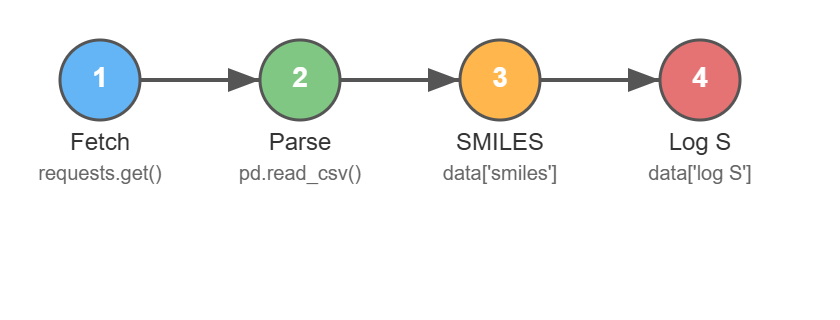
Result Interpretation:
Dataset contains 1128 molecules
Solubility range: -11.60 to 1.58 log S
What do these numbers mean?
- log S = –11.60 → Solubility = $10^{-11.60}$ mol/L (extremely insoluble)
- log S = 1.58 → Solubility = $10^{1.58}$ mol/L (very soluble)
- Range: 13.18 log units = $10^{13.18}$ ≈ 15 trillion-fold difference!
In Real-World Context:
- Very soluble (log S > 0): Like sugar in water – dissolves easily
- Moderately soluble (–3 < log S < 0): Like alcohol – mixes well
- Poorly soluble (log S < –3): Like oil – forms a separate layer
- Practically insoluble (log S < –6): Like plastic – never dissolves
Step 2.2: Examining Example Molecules
Let’s examine some specific molecules to understand the dataset diversity:
| Data Exploration Process | ||
|---|---|---|
|
Purpose: Understand dataset Check molecular diversity |
Method: Print first 5 molecules SMILES + solubility |
Insight: Complexity varies Simple to complex structures |
print("\nExample molecules from the dataset:")
print("-" * 60)
print(f"{'SMILES':<40} {'Solubility (log S)':<20}")
print("-" * 60)

for i in range(5):
    print(f"{smiles_list[i]:<40} {solubility_values[i]:<20.2f}")
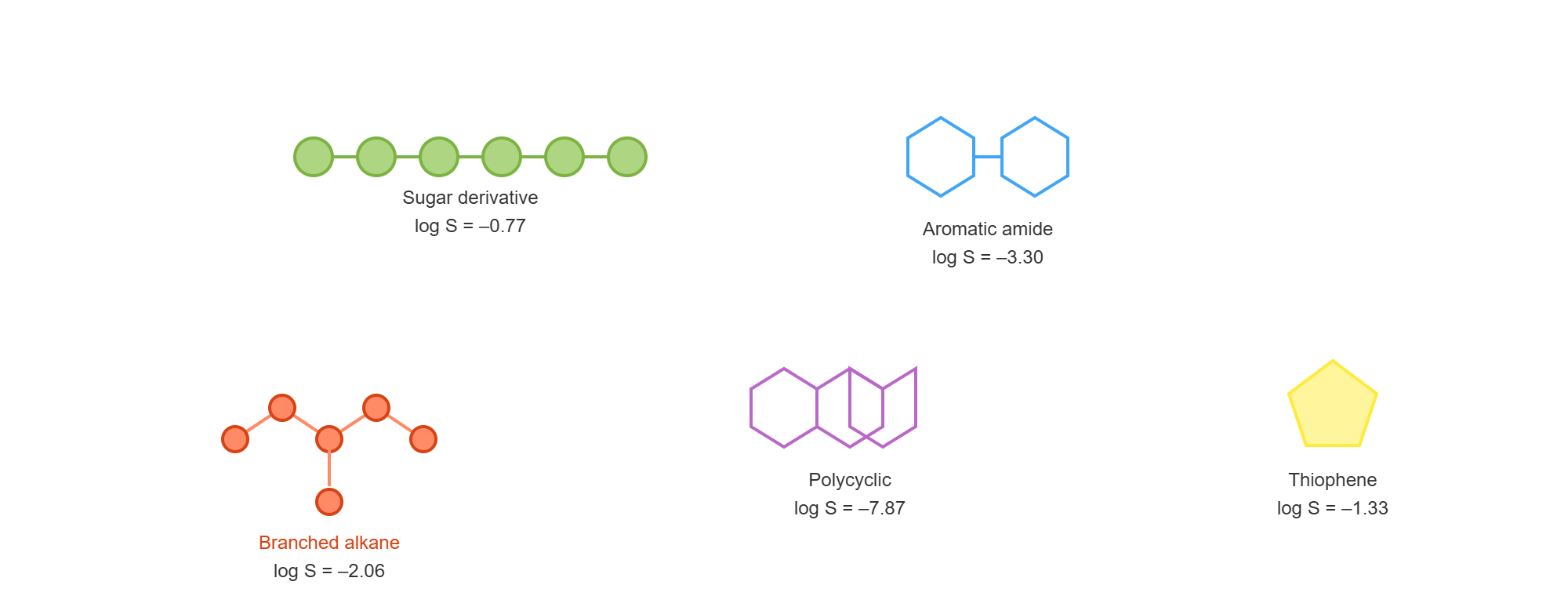
Result Interpretation:
Example molecules from the dataset:
------------------------------------------------------------
SMILES                                   Solubility (log S)
------------------------------------------------------------
OCC3OC(OCC2OC(OC(C#N)c1ccccc1)C(O)C(O)C2O)C(O)C(O)C3O  -0.77
Cc1occc1C(=O)Nc2ccccc2                   -3.30
CC(C)=CCCC(C)=CC(=O)                     -2.06
c1ccc2c(c1)ccc3c2ccc4c5ccccc5ccc43       -7.87
c1ccsc1                                  -1.33
Chemical Interpretation:
- Row 1: Complex sugar derivative with multiple –OH groups → relatively soluble (log S = –0.77)
- Row 4: Large polycyclic aromatic hydrocarbon → very insoluble (log S = –7.87)
- Row 5: Small thiophene heterocycle → moderate solubility (log S = –1.33)
The dataset covers a wide range of molecular complexity and functional groups.
Step 2.3: Visualizing Solubility Distribution
Understanding the distribution helps us assess potential modeling challenges:
| Visualization Purpose | ||
|---|---|---|
|
What: Histogram of solubility 50 bins |
Why: See data distribution Identify skewness |
Insight: Most molecules poorly soluble Left-skewed distribution |
plt.figure(figsize=(10, 6))
plt.hist(solubility_values, bins=50, edgecolor='black', alpha=0.7)
plt.xlabel('Log Solubility (log S)', fontsize=12)
plt.ylabel('Count', fontsize=12)
plt.title('Distribution of Solubility Values in ESOL Dataset', fontsize=14)
plt.grid(True, alpha=0.3)
plt.show()
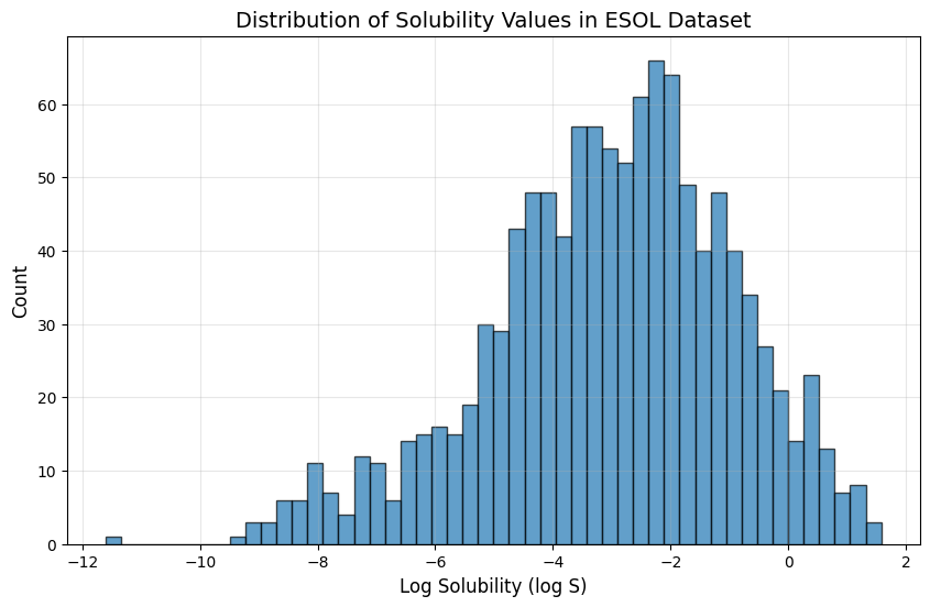
Result Interpretation:
- Central tendency: Distribution peaks around -2 to -3 log S
- Skewness: Left-skewed distribution (more insoluble molecules)
- Chemical reality: Most organic molecules have limited water solubility
- Modeling implication: Model may perform better on common solubility ranges than extremes
Step 3: Converting Molecules to Graph Representations
Step 3.1: Testing Feature Extraction on Water
We validate our feature extraction by testing on water (H₂O), the simplest molecule:
| Water Molecule Test Process | |||
|---|---|---|---|
|
Input: SMILES: "O" Oxygen only |
Step 1: Parse SMILES Create mol object |
Step 2: Add H atoms O → H-O-H |
Step 3: Extract features For O, H, H |
# Parse water molecule
water_smiles = "O"
water = Chem.MolFromSmiles(water_smiles)
water = Chem.AddHs(water)  # Add explicit hydrogens

print("Water molecule (H2O) atom features:")
print("-" * 50)
for i, atom in enumerate(water.GetAtoms()):
    features = get_atom_features(atom)
    symbol = atom.GetSymbol()
    print(f"Atom {i} ({symbol}): {features}")
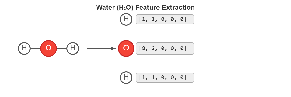
Result Interpretation:
Water molecule (H2O) atom features:
--------------------------------------------------
Atom 0 (O): [8, 2, 0, 0, 0]
Atom 1 (H): [1, 1, 0, 0, 0]
Atom 2 (H): [1, 1, 0, 0, 0]
Feature Vector Breakdown:
Oxygen: [8, 2, 0, 0, 0]
- 8 = Atomic number (element oxygen)
- 2 = Degree (bonded to 2 hydrogen atoms)
- 0 = No formal charge (neutral)
- 0 = Not aromatic (water is not aromatic)
- 0 = No implicit hydrogens (all are explicit)
Hydrogen: [1, 1, 0, 0, 0]
- 1 = Atomic number (element hydrogen)
- 1 = Degree (bonded to 1 oxygen atom)
- Remaining features are all zero
Step 3.2: Testing Bond Extraction on Ethanol
Test on a more complex molecule to see bond connectivity:
| Ethanol Bond Analysis | ||
|---|---|---|
|
Molecule: Ethanol (CCO) CH₃-CH₂-OH |
Expected: 9 atoms total 2C + 1O + 6H |
Bonds: 8 undirected 16 directed edges |
# Test on ethanol
ethanol_smiles = "CCO"
ethanol = Chem.MolFromSmiles(ethanol_smiles)
ethanol = Chem.AddHs(ethanol)

connections = get_bond_connections(ethanol)

print(f"Ethanol molecule (C2H6O):")
print(f"  Number of atoms: {ethanol.GetNumAtoms()}")
print(f"  Number of bonds: {len(connections)//2}")
print(f"  Number of directed edges: {len(connections)}")
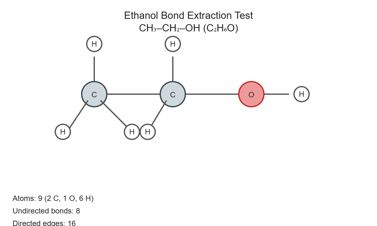
Result:
Ethanol molecule (C2H6O):
  Number of atoms: 9
  Number of bonds: 8
  Number of directed edges: 16
Step 3.3: Detailed Edge Analysis
| Edge Directionality Explanation | |
|---|---|
|
Why Bidirectional? • Electrons flow both ways • Message passing needs it • Reflects chemical reality |
Example: C-C bond becomes: • Edge 0: C→C • Edge 1: C←C |
print("\nFirst few connections (atom index pairs):")
for i, (src, dst) in enumerate(connections[:6]):
    src_symbol = ethanol.GetAtomWithIdx(src).GetSymbol()
    dst_symbol = ethanol.GetAtomWithIdx(dst).GetSymbol()
    print(f"  Edge {i}: {src}({src_symbol}) → {dst}({dst_symbol})")
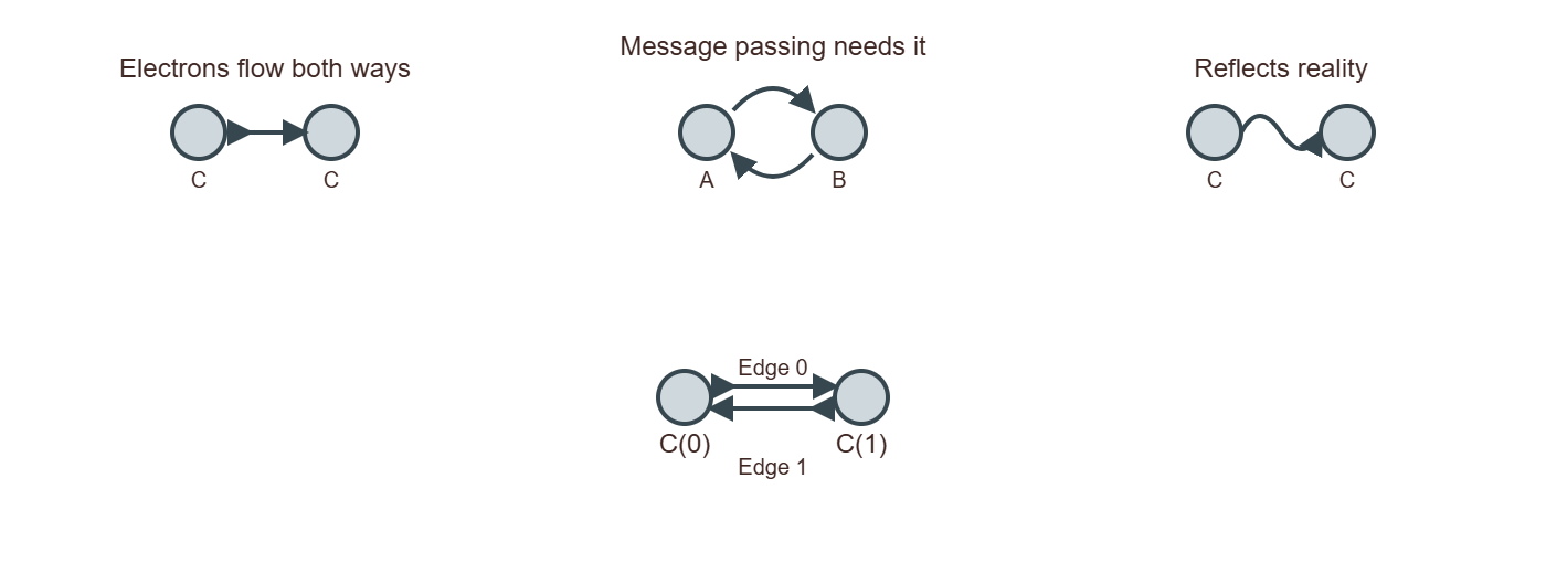
Result:
First few connections (atom index pairs):
  Edge 0: 0(C) → 1(C)
  Edge 1: 1(C) → 0(C)
  Edge 2: 1(C) → 2(O)
  Edge 3: 2(O) → 1(C)
  Edge 4: 0(C) → 3(H)
  Edge 5: 3(H) → 0(C)
Chemical Interpretation: Each bond appears twice (e.g., C→C and C←C) to enable bidirectional message passing in the GNN. This reflects the quantum mechanical reality that electrons are shared between atoms.
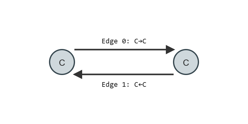
Step 3.4: Complete Molecule-to-Graph Conversion
Implementation Strategy:
| Step | Process | Output |
|---|---|---|
| 1 | SMILES String → RDKit Molecule | Molecule object |
| 2 | Add Hydrogens | Complete molecule |
| 3 | Extract Features | Node feature matrix |
| 4 | Extract Bonds | Edge index |
| 5 | Create PyG Data | Graph object |
| Main Conversion Function Structure | |
|---|---|
|
Function Inputs: • SMILES string • Solubility value (optional) |
Function Outputs: • PyG Data object • None if parsing fails |
|
Processing Steps: Parse → Add H → Extract features → Extract bonds → Package |
|
def molecule_to_graph(smiles, solubility=None):
    """
    Complete pipeline: SMILES → Molecular Graph

    Uses RDKit for chemistry, PyTorch Geometric for graph structure
    """
    # Parse SMILES
    mol = Chem.MolFromSmiles(smiles)
    if mol is None:
        return None

    # Add hydrogens (affects H-bonding)
    mol = Chem.AddHs(mol)
Step 3.4.1: Feature Extraction Part
| Feature Extraction Loop | ||
|---|---|---|
|
For each atom: Call get_atom_features() Returns list of 5 numbers |
Collect all: atom_features list [[f1], [f2], ...] |
Convert: To PyTorch tensor Shape: [n_atoms, 5] |
    # Extract atom features
    atom_features = []
    for atom in mol.GetAtoms():
        atom_features.append(get_atom_features(atom))

    # Convert to tensor
    x = torch.tensor(atom_features, dtype=torch.float)
Step 3.4.2: Edge Construction Part
| Edge Index Construction | ||
|---|---|---|
|
Get bonds: Call get_bond_connections Returns [[i,j], ...] |
Handle edge case: Single atoms Add self-loop [0,0] |
Format for PyG: Transpose to COO Shape: [2, n_edges] |
    # Extract bonds
    edge_list = get_bond_connections(mol)
    if len(edge_list) == 0:  # Single atom
        edge_list = [[0, 0]]  # Self-loop

    # Create edge index (transpose for PyG format)
    edge_index = torch.tensor(edge_list, dtype=torch.long).t().contiguous()
Step 3.4.3: Data Object Creation
| PyG Data Object Assembly | |
|---|---|
|
Required fields: • x: node features • edge_index: connectivity |
Optional fields: • y: target value • Other properties |
    # Create Data object
    data = Data(x=x, edge_index=edge_index)

    # Add label if provided
    if solubility is not None:
        data.y = torch.tensor([solubility], dtype=torch.float)

    return data
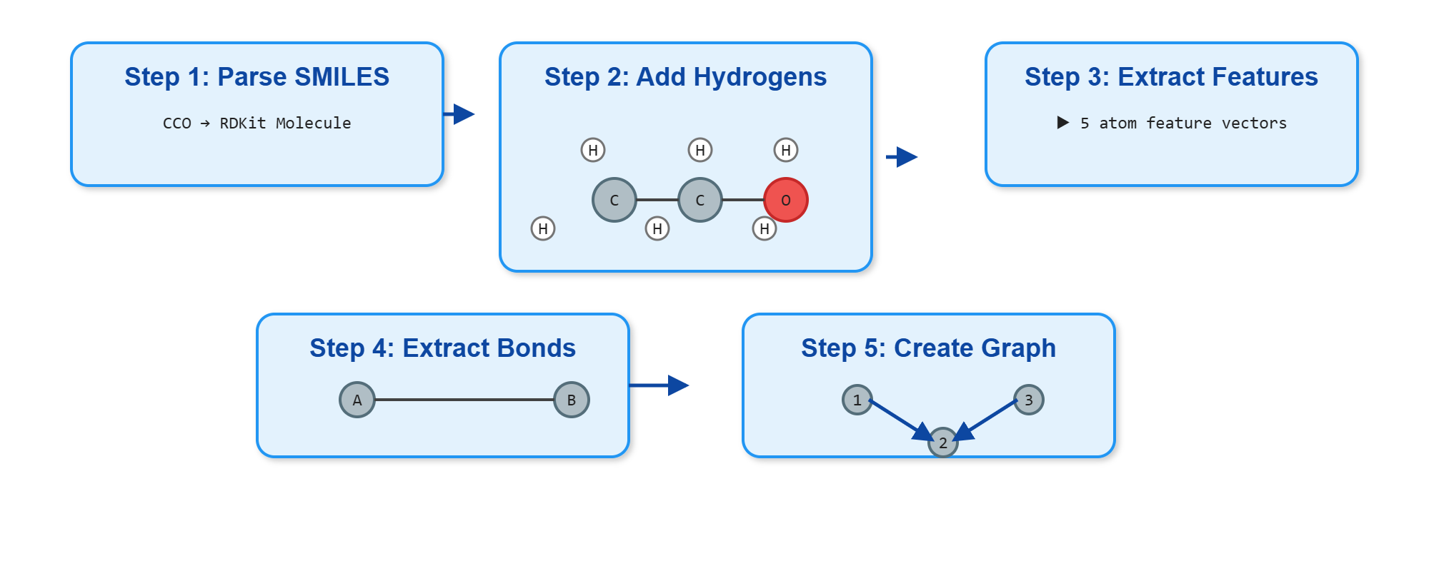
Step 3.5: Testing the Conversion Pipeline
Test on molecules of varying complexity:
| Test Strategy | ||
|---|---|---|
|
Test 1: Water (O) 3 atoms, 2 bonds |
Test 2: Ethanol (CCO) 9 atoms, 8 bonds |
Test 3: Benzene (c1ccccc1) 12 atoms, 12 bonds |
test_molecules = [
    ("O", "Water"),
    ("CCO", "Ethanol"),
    ("c1ccccc1", "Benzene")
]

print("Testing molecule to graph conversion:")
print("-" * 60)

for smiles, name in test_molecules:
    graph = molecule_to_graph(smiles, solubility=0.0)
    if graph:
        print(f"{name} ({smiles}):")
        print(f"  Atoms: {graph.x.shape[0]}")
        print(f"  Features per atom: {graph.x.shape[1]}")
        print(f"  Bonds: {graph.edge_index.shape[1] // 2}")
        print(f"  Graph object: {graph}")
        print()
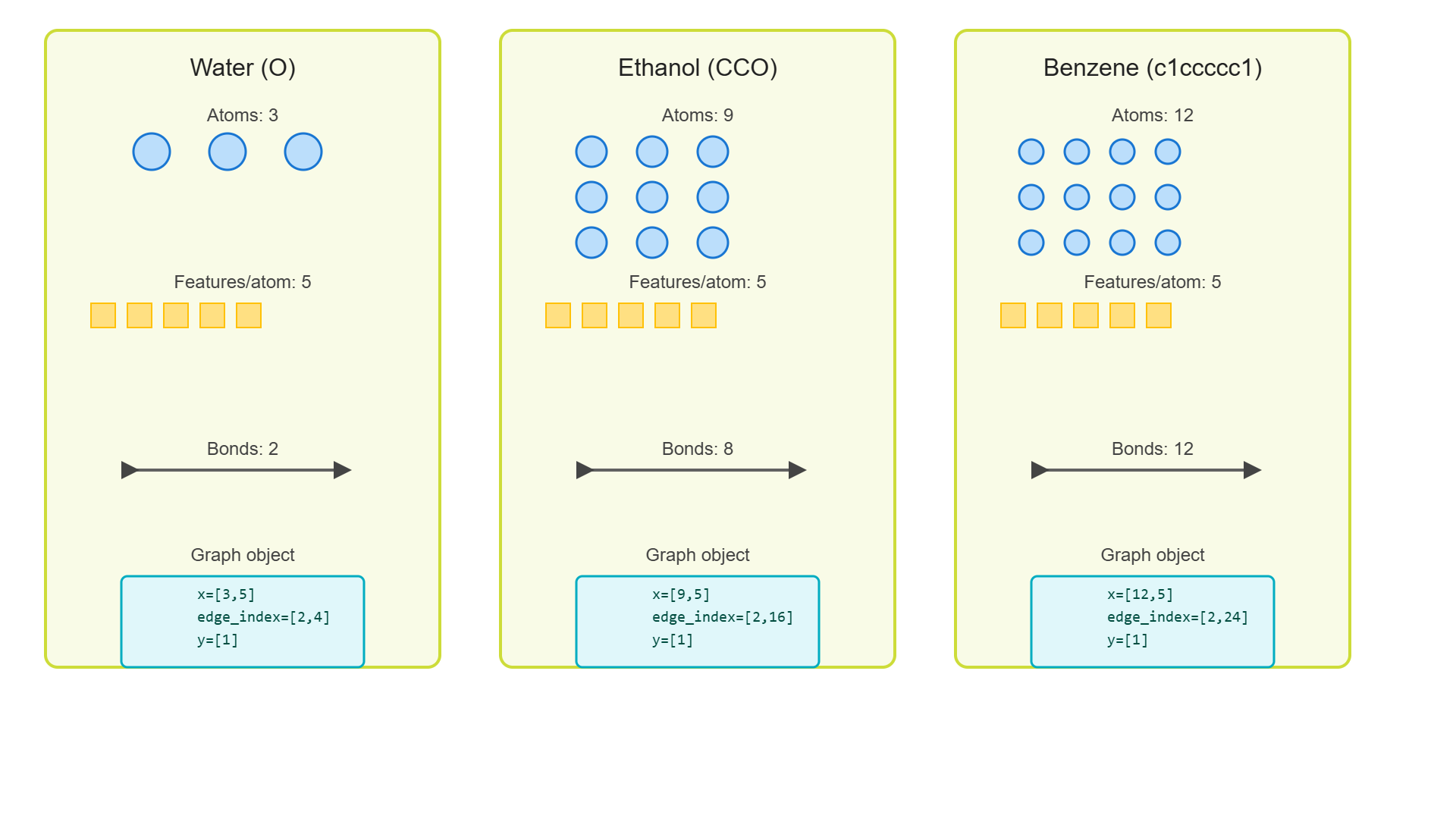
Result Interpretation:
Testing molecule to graph conversion:
------------------------------------------------------------
Water (O):
  Atoms: 3
  Features per atom: 5
  Bonds: 2
  Graph object: Data(x=[3, 5], edge_index=[2, 4], y=[1])

Ethanol (CCO):
  Atoms: 9
  Features per atom: 5
  Bonds: 8
  Graph object: Data(x=[9, 5], edge_index=[2, 16], y=[1])

Benzene (c1ccccc1):
  Atoms: 12
  Features per atom: 5
  Bonds: 12
  Graph object: Data(x=[12, 5], edge_index=[2, 24], y=[1])
How to interpret “Data(x=[12, 5], edge_index=[2, 24], y=[1])” ?
- x: Node feature matrix
[num_atoms, num_features] - edge_index: COO-format edges
[2, num_edges] - y: Target property (solubility)
Example – Benzene:
- 6 carbon atoms + 6 hydrogen atoms = 12 nodes
- 6 C–C bonds + 6 C–H bonds = 12 undirected bonds
- 12 undirected bonds × 2 directions = 24 directed edges
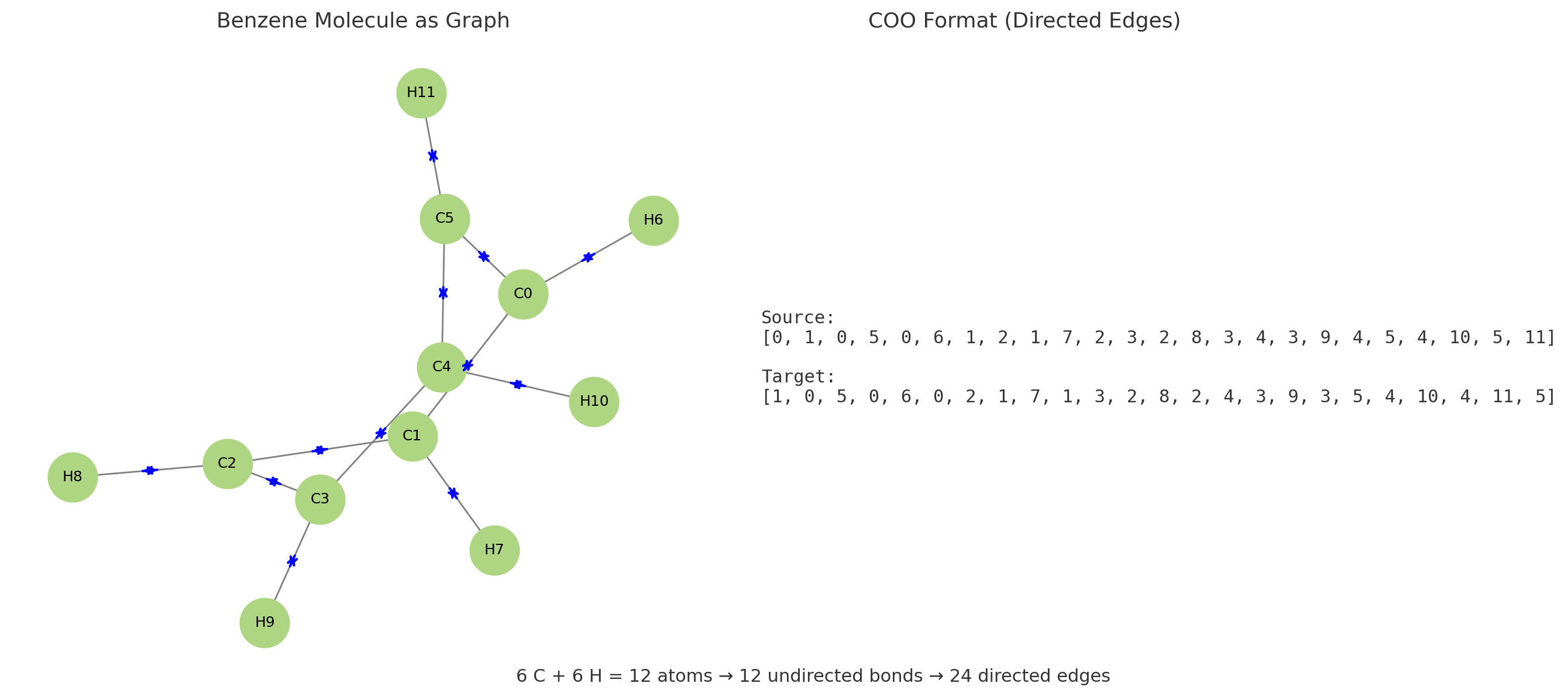
What is COO Format? COO (COOrdinate) format stores edges as pairs of node indices:
- First row: source nodes
[0, 1, 1, 2, …] - Second row: target nodes
[1, 0, 2, 1, …] - Each column is one edge:
(0→1),(1→0),(1→2),(2→1), …
Step 4: Building the Graph Neural Network Architecture
Step 4.1: Review the GNN Design Principles
Message Passing Framework: As we have seen before, each GCN layer performs the following operation:
\[h_i^{(l+1)} = \sigma\bigl(W^{(l)} \cdot \mathrm{AGG}(\{h_j^{(l)} : j \in N(i) \cup \{i\}\})\bigr)\]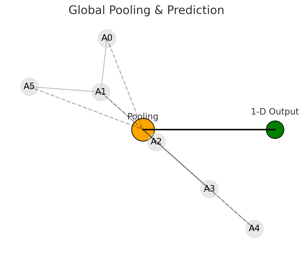
Breaking Down This Formula
- $h_i^{(l)}$ — What atom i knows at layer l
- $N(i)$ — Atom i’s neighbors (bonded atoms)
- $\mathrm{AGG}()$ — Combine information from neighbors (usually average)
- $W^{(l)}$ — Learnable transformation (the “smart” part)
- $\sigma$ — Activation function (adds non-linearity)
Step 4.2: Set up the Model Architecture
| Design Choices | Architecture Intuition |
|---|---|
| 3 GCN layers | Why 3 layers? Most chemical effects happen within 3 bonds. Captures 3-hop neighborhoods (sufficient for most molecular patterns) |
| 64 hidden dimensions | Why 64 dimensions? Enough to capture complexity, not too much to overfit. Balances expressiveness vs overfitting |
| Global mean pooling | Why mean pooling? Average all atom features to get molecule feature. Aggregates variable-sized molecules to fixed representation |
| Single output | Final value is log solubility — a continuous target. Predicts scalar solubility value |
Step 4.3: Class Definition and Initialization
| Model Architecture Components | ||
|---|---|---|
|
Component 1: GCN Layers 3 layers in ModuleList |
Component 2: Predictor Linear layer (64→1) |
Flow: Atoms→GCN→Pool→Predict Variable→Fixed size |
class MolecularGNN(nn.Module):
    """
    Graph Neural Network for molecular property prediction

    Architecture Flow:
    Atoms (5 features) → GCN layers → Molecular embedding (64) → Solubility (1)
    """

    def __init__(self, num_features=5, hidden_dim=64, num_layers=3):
        super(MolecularGNN, self).__init__()

        self.num_features = num_features
        self.hidden_dim = hidden_dim
        self.num_layers = num_layers

        # Build GCN layers
        self.convs = nn.ModuleList()
Step 4.3.1: Layer Construction
| Layer Construction Process | ||
|---|---|---|
|
Layer 1: Input → Hidden 5 features → 64 dims |
Layers 2-3: Hidden → Hidden 64 dims → 64 dims |
Output Layer: Hidden → Prediction 64 dims → 1 value |
        # First layer: 5 → 64
        self.convs.append(GCNConv(num_features, hidden_dim))

        # Hidden layers: 64 → 64
        for _ in range(num_layers - 1):
            self.convs.append(GCNConv(hidden_dim, hidden_dim))

        # Output layer: 64 → 1
        self.predictor = nn.Linear(hidden_dim, 1)
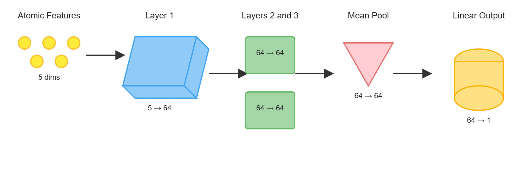
Step 4.3.2: Forward Pass Implementation
Principle: The forward pass implements message passing followed by pooling:
| Forward Pass Flow | |||
|---|---|---|---|
|
Step 1: Message Passing 3 GCN layers |
Step 2: Activation ReLU after each |
Step 3: Pooling Atoms → Molecule |
Step 4: Prediction 64 → 1 value |
    def forward(self, x, edge_index, batch):
        """
        Forward propagation through GNN

        Args:
            x: Node features [num_atoms_in_batch, 5]
            edge_index: Edge connectivity [2, num_edges_in_batch]
            batch: Maps atoms to molecules [num_atoms_in_batch]
        """
        # Message passing layers
        for conv in self.convs:
            x = conv(x, edge_index)
            x = F.relu(x)  # Non-linearity

        # Aggregate atoms → molecules
        x = global_mean_pool(x, batch)

        # Predict property
        return self.predictor(x)
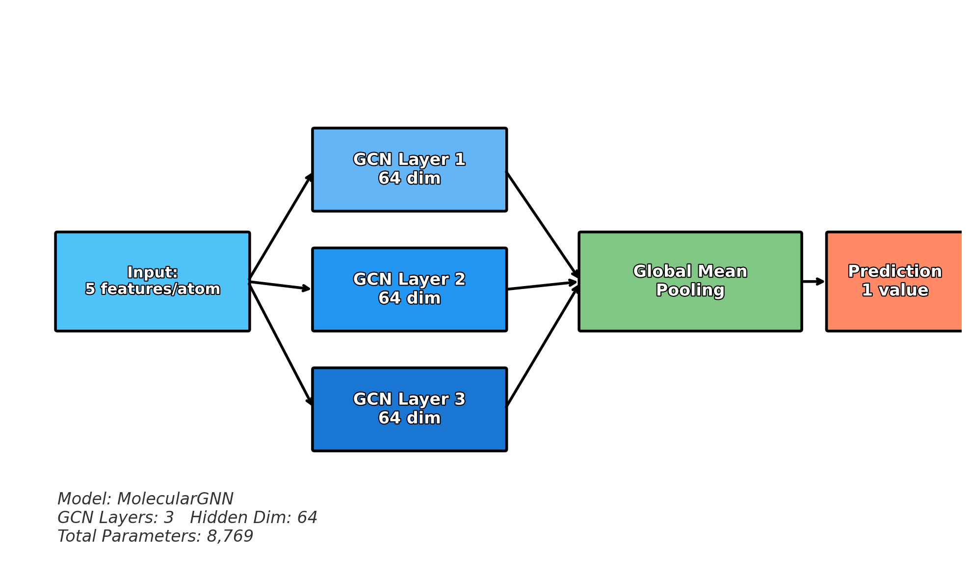
What Actually Happens in Forward Pass?
- Input: Each atom starts with 5 features
- Layer 1: Atoms exchange info with neighbors, transform to 64 features
- Layer 2: Exchange again, refine understanding
- Layer 3: Final exchange, atoms now “know” their 3-hop neighborhood
- Pooling: Average all atoms to get one molecule representation
- Prediction: Transform 64 features to 1 solubility value
Key Point: The network learns what information to exchange and how to transform it!
Step 4.4: Model Analysis
Let’s analyze the model architecture:
| Model Analysis Process | |
|---|---|
|
What we're doing: • Create model instance • Count parameters • Analyze complexity |
Why it matters: • Understand model size • Compare to other DNNs • Check if overfitting risk |
# Create model instance
model = MolecularGNN(num_features=5, hidden_dim=64, num_layers=3)

# Count parameters
total_params = sum(p.numel() for p in model.parameters())
print(f"Model architecture: MolecularGNN")
print(f"  Input features: 5 (per atom)")
print(f"  Hidden dimension: 64")
print(f"  Number of GCN layers: 3")
print(f"  Total parameters: {total_params:,}")
Result:
Model architecture: MolecularGNN
  Input features: 5 (per atom)
  Hidden dimension: 64
  Number of GCN layers: 3
  Total parameters: 8,769
Step 4.5: Detailed Parameter Breakdown
| Parameter Breakdown Analysis | |
|---|---|
|
Purpose: See where parameters are Weights vs biases |
Insight: Most params in hidden layers 64×64 = 4096 each |
print("\nLayer-by-layer breakdown:")
for name, param in model.named_parameters():
    print(f"  {name}: {param.shape}")
Result:
Layer-by-layer breakdown:
  convs.0.bias: torch.Size([64])
  convs.0.lin.weight: torch.Size([64, 5])
  convs.1.bias: torch.Size([64])
  convs.1.lin.weight: torch.Size([64, 64])
  convs.2.bias: torch.Size([64])
  convs.2.lin.weight: torch.Size([64, 64])
  predictor.weight: torch.Size([1, 64])
  predictor.bias: torch.Size([1])
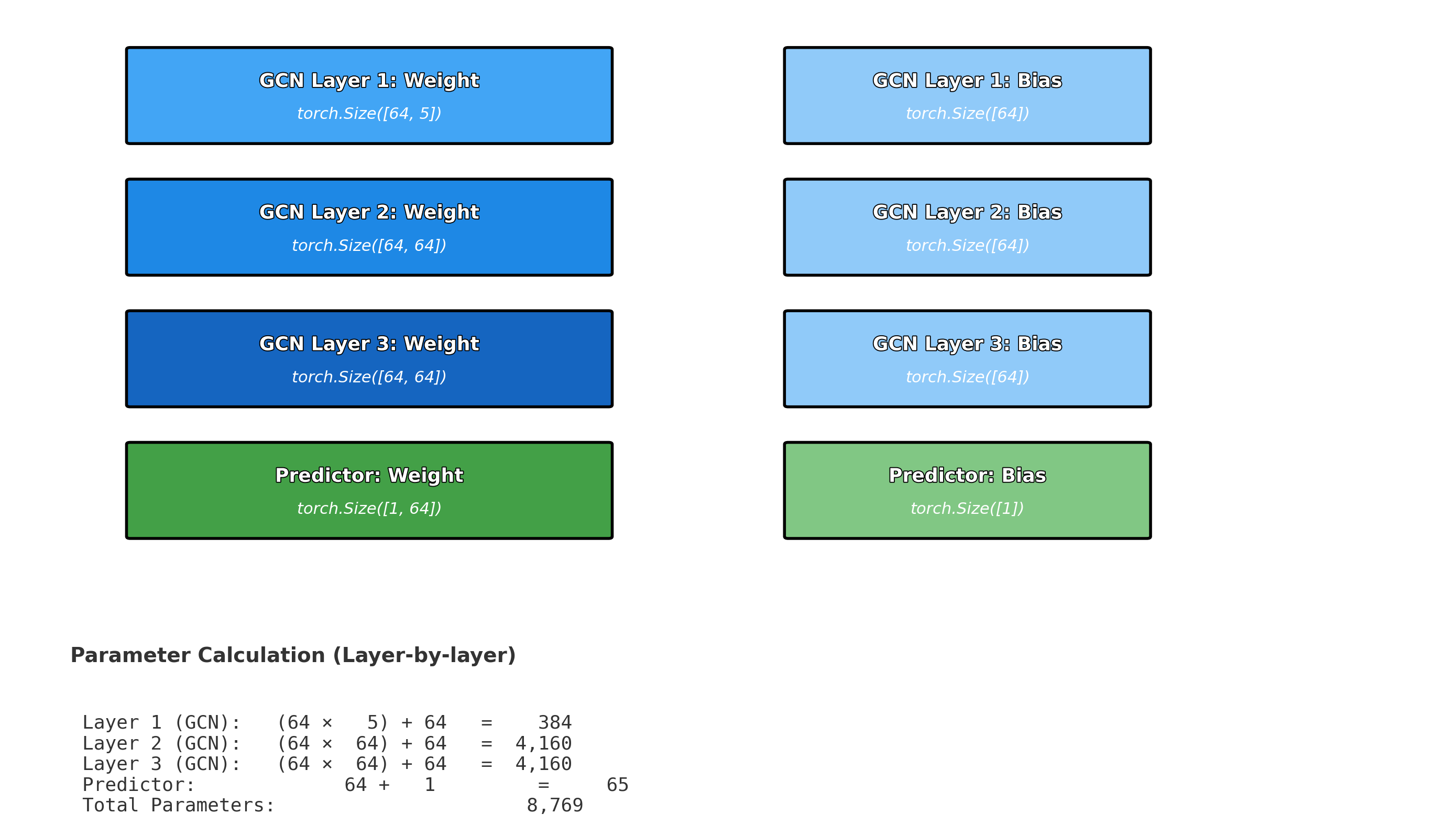
Step 5: Preparing Training Data
Step 5.1: Dataset Conversion
Convert all molecules to graphs, handling potential failures:
| Dataset Conversion Pipeline | |||
|---|---|---|---|
|
Step 1: Loop molecules 1000 total |
Step 2: Convert each SMILES → Graph |
Step 3: Handle failures Track bad SMILES |
Result: List of graphs Ready for training |
num_molecules = 1000  # Use subset for faster training
graphs = []
failed_molecules = []

print(f"Converting {num_molecules} molecules to graphs...")

for i in range(num_molecules):
    smiles = smiles_list[i]
    solubility = solubility_values[i]

    graph = molecule_to_graph(smiles, solubility)
    if graph is not None:
        graphs.append(graph)
    else:
        failed_molecules.append((i, smiles))
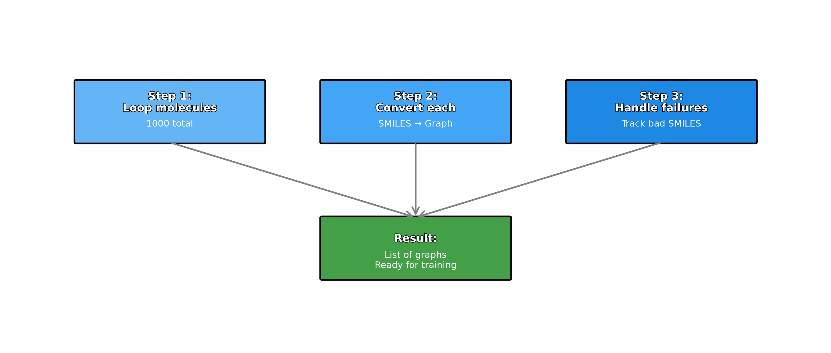
Conversion Results:
| Conversion Quality Check | |
|---|---|
|
Success Rate: 100% (1000/1000) All SMILES valid |
Meaning: High quality dataset Well-curated ESOL |
print(f"Successfully converted: {len(graphs)} molecules")
print(f"Failed conversions: {len(failed_molecules)} molecules")
Result:
Converting 1000 molecules to graphs...
Successfully converted: 1000 molecules
Failed conversions: 0 molecules
100% success rate indicates high-quality SMILES strings in the ESOL dataset. RDKit successfully parsed all molecules.
Step 5.2: Train-Test Split
Always evaluate on unseen data to assess generalization. We use 80/20 split:
| Train-Test Split Strategy | ||
|---|---|---|
|
Training Set (80%): 800 molecules Model learns from these |
Test Set (20%): 200 molecules Never seen during training |
Purpose: Prevent overfitting Test generalization |
# 80/20 split (standard in ML)
train_size = int(0.8 * len(graphs))
train_graphs = graphs[:train_size]
test_graphs = graphs[train_size:]

print(f"\nDataset split:")
print(f"  Training: {len(train_graphs)} molecules")
print(f"  Testing: {len(test_graphs)} molecules")
Result:
Dataset split:
  Training: 800 molecules
  Testing: 200 molecules
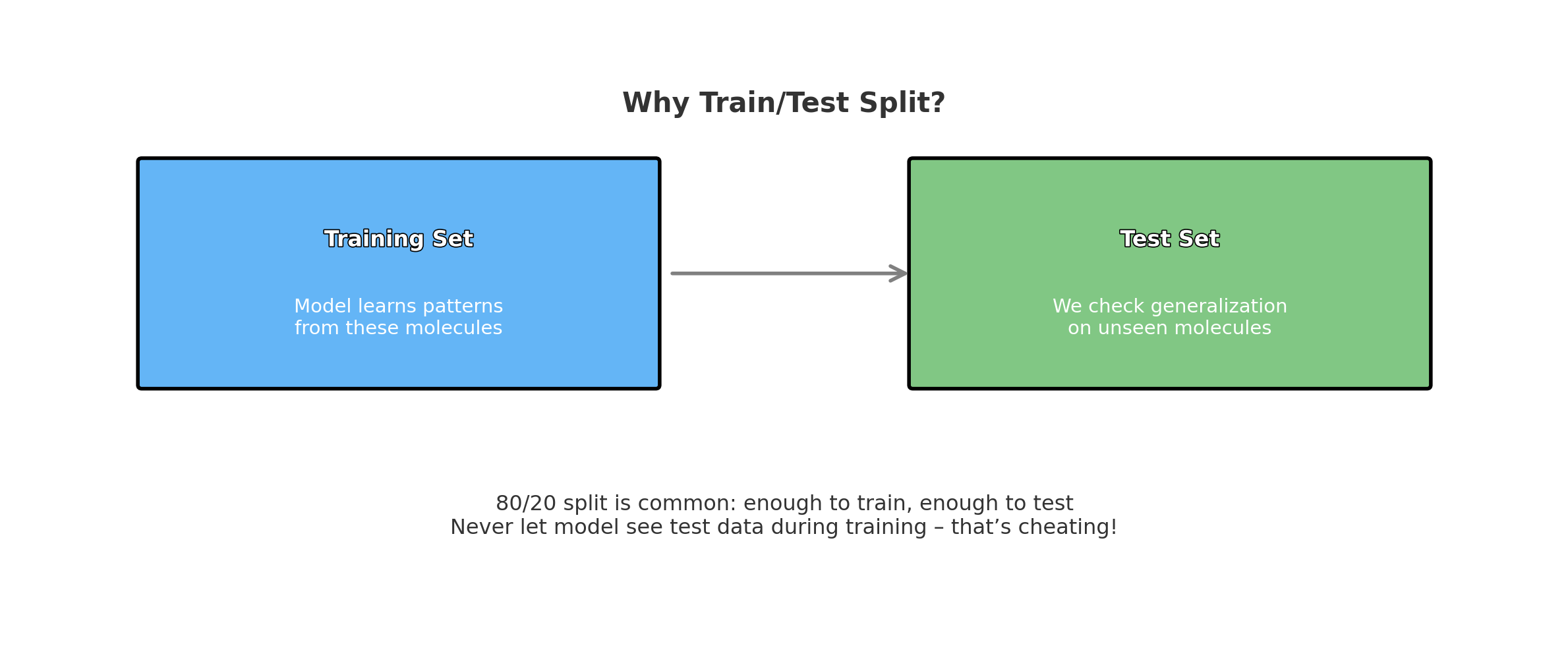
Step 5.3: Creating DataLoaders
DataLoader automatically batches variable-sized graphs:
| DataLoader Configuration | ||
|---|---|---|
|
Batch Size: 32 molecules/batch Process together |
Shuffle: True for training Random order helps |
Result: 25 train batches 7 test batches |
# Batch size 32 is typical for molecular property prediction
train_loader = DataLoader(train_graphs, batch_size=32, shuffle=True)
test_loader = DataLoader(test_graphs, batch_size=32, shuffle=False)

print(f"Data loaders created:")
print(f"  Training batches: {len(train_loader)}")
print(f"  Test batches: {len(test_loader)}")
print(f"  Batch size: 32")
Result:
Data loaders created:
  Training batches: 25
  Test batches: 7
  Batch size: 32
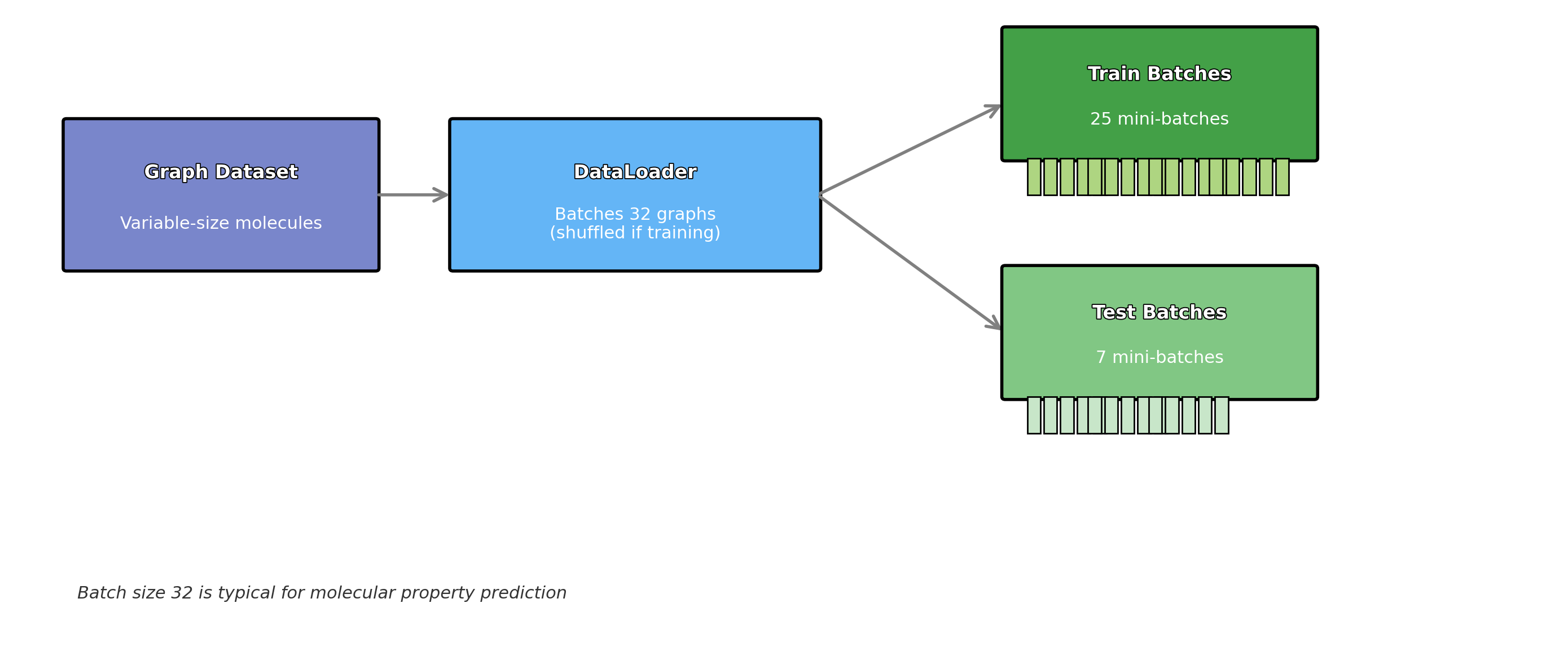
Step 5.4: Batch Structure Analysis:
| Understanding Batch Structure | |
|---|---|
|
Challenge: Molecules have different sizes • Water: 3 atoms • Aspirin: 21 atoms How to batch? |
Solution: Combine into one big graph • All atoms together • Batch tensor tracks ownership • No edges between molecules |
# Inspect batch structure
for batch in train_loader:
    print(f"\nExample batch:")
    print(f"  Total atoms in batch: {batch.x.shape[0]}")
    print(f"  Total molecules in batch: {batch.num_graphs}")
    print(f"  Batch tensor shape: {batch.batch.shape}")
    print(f"  Edge index shape: {batch.edge_index.shape}")
    break
Result:
Example batch:
  Total atoms in batch: 864
  Total molecules in batch: 32
  Batch tensor shape: torch.Size([864])
  Edge index shape: torch.Size([2, 1744])
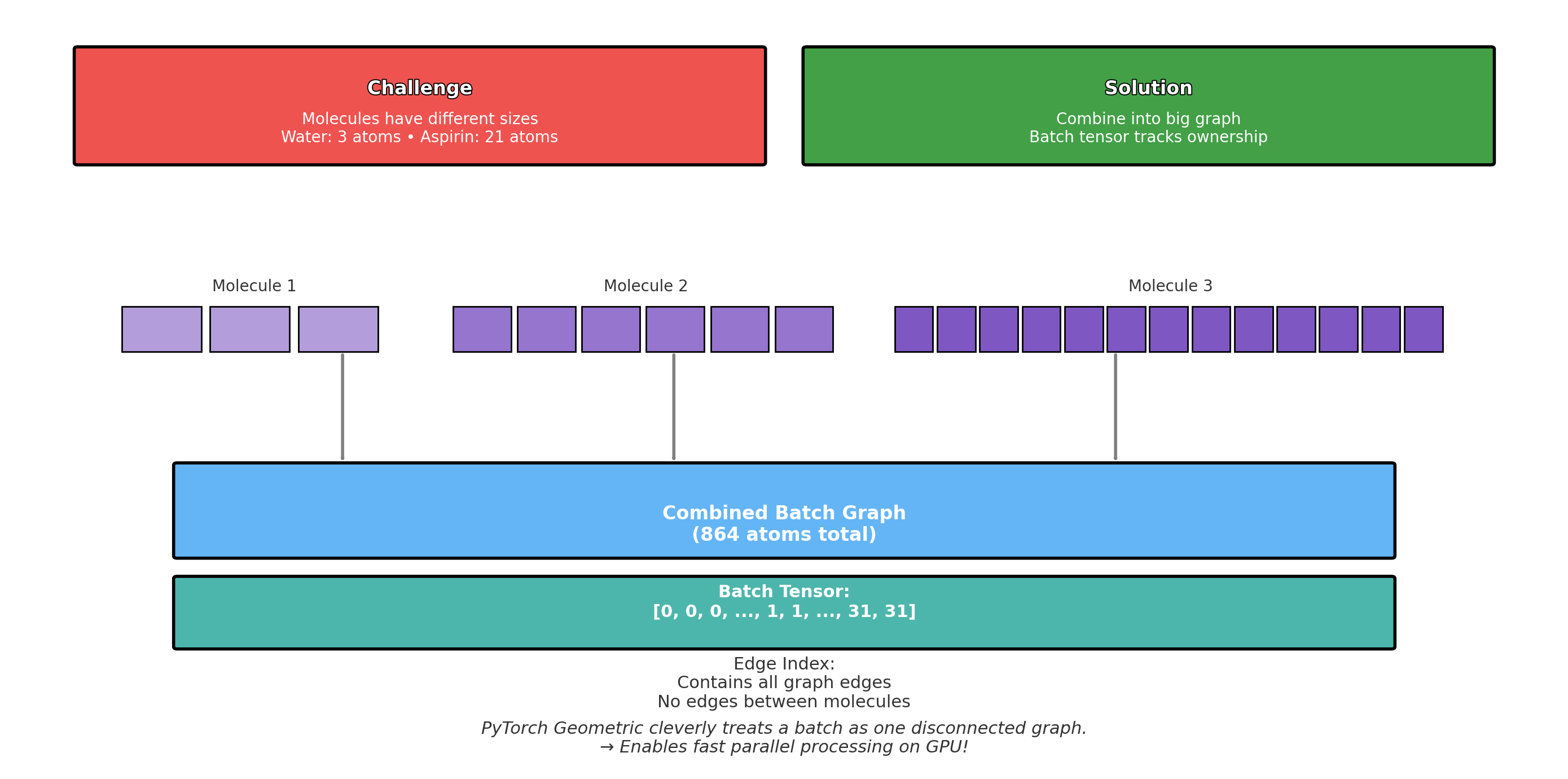
Batching Mechanism Explained:
-
32 molecules contain 864 atoms total (average ≈ 27 atoms/molecule)
-
Batch tensor:
[0, 0, 0, ..., 1, 1, 1, ..., 31, 31, 31]Maps each atom to its parent molecule (0–31)
-
Edge index combines all molecular graphs into one large disconnected graph
-
Enables efficient parallel processing on GPU
After combination, PyTorch Geometric treats a batch of graphs as one big disconnected graph!
- Molecule 1: atoms 0–20
- Molecule 2: atoms 21–35
- No edges between molecules
- Process all at once = FAST!
Step 6: Training the Model
Step 6.1: Training Components Setup
Step 6.1.1: Adam Optimizer Combines momentum with adaptive learning rates
\[\begin{aligned} m_t &= \beta_1 m_{t-1} + (1 - \beta_1)\,g_t \\ v_t &= \beta_2 v_{t-1} + (1 - \beta_2)\,g_t^2 \\ \theta_t &= \theta_{t-1} - \alpha\,\frac{m_t}{\sqrt{v_t + \epsilon}} \end{aligned}\]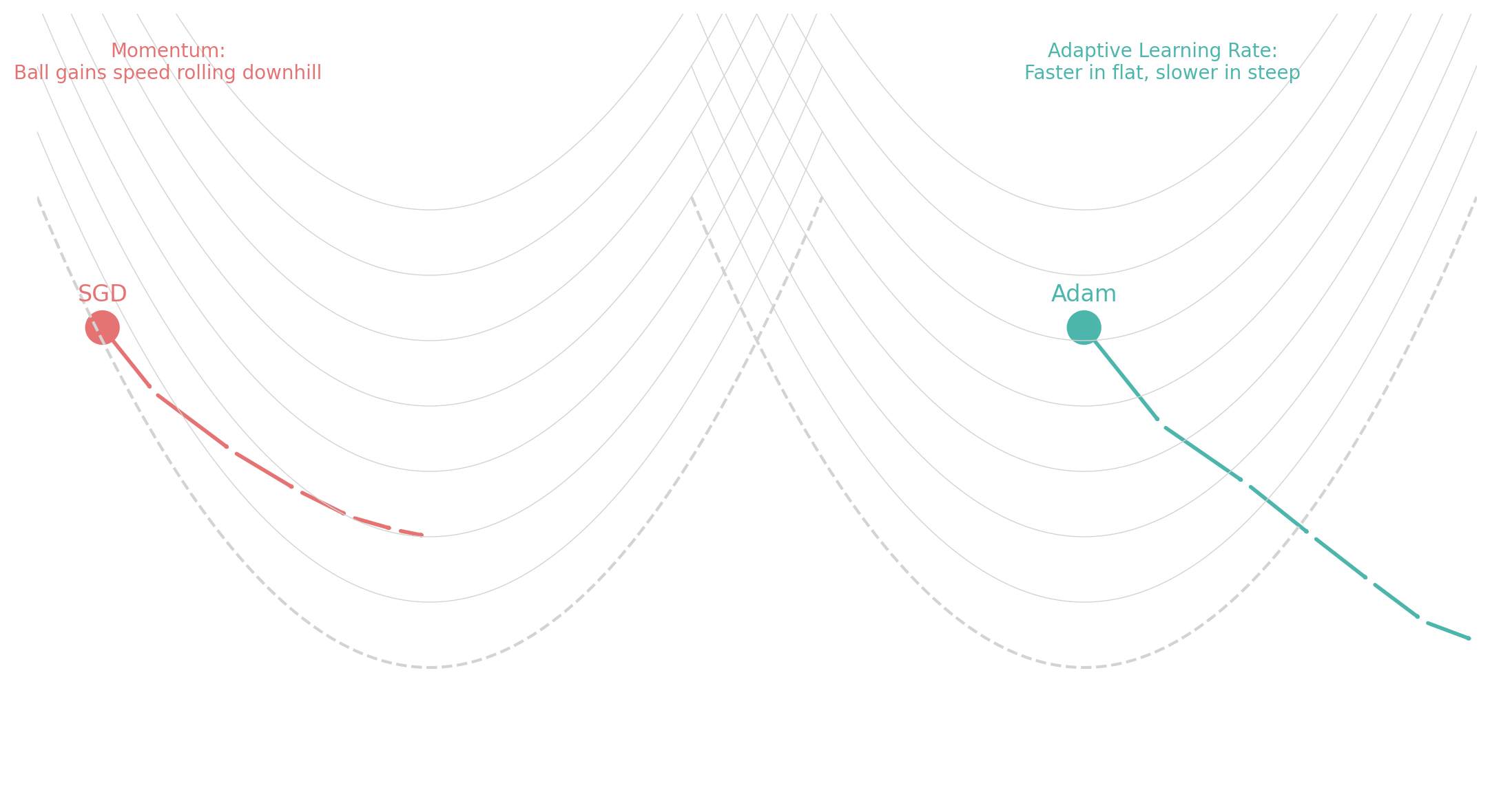
-
$m_t$ (Momentum):
\[m_t = \beta_1 m_{t-1} + (1 - \beta_1) g_t\]
This term computes an exponential moving average of the gradients. It combines the current gradient $g_t$ with the historical average $m_{t-1}$:Think of it as “smoothing out” the direction of updates. Instead of reacting to each new gradient immediately, $m_t$ helps the model maintain a stable direction over time.
Imagine pushing a ball downhill: the more consistent the slope, the faster it builds momentum. Similarly, $m_t$ gives you an accumulated sense of which direction consistently reduces the loss. -
$v_t$ (Adaptive scaling):
\[v_t = \beta_2 v_{t-1} + (1 - \beta_2) g_t^2\]
This term accumulates the squared gradients to estimate how large and volatile each parameter’s updates are:Unlike $m_t$, $v_t$ only tracks the magnitude of the gradients (not their direction). It tells you whether the updates for a certain parameter dimension have been large or small recently.
If a direction has large or noisy gradients, $v_t$ becomes large, and the update will be smaller in that direction. Think of it as driving over bumpy terrain: the bumpier it is, the more cautiously you move forward. -
$\theta_t$ (Final update):
\[\theta_t = \theta_{t-1} - \alpha \cdot \frac{m_t}{\sqrt{v_t} + \epsilon}\]
This is the final step that uses both $m_t$ and $v_t$ to update the model parameters:The numerator ($m_t$) tells you which direction to move, and the denominator ($\sqrt{v_t}$) controls how big the step should be in that direction.
If $v_t$ is large (unstable or steep), the denominator increases, shrinking the step size. If $v_t$ is small (smooth), the update is larger.
The learning rate $\alpha$ scales the entire step size globally (e.g., 0.001), while $\epsilon$ is a small number added for numerical stability.This adaptive combination makes Adam very effective in complex landscapes — it balances speed and caution, moving quickly in flat regions and slowly where gradients are volatile.
Step 6.1.2: MSE Loss For regression tasks
\[L = \frac{1}{n} \sum_{i=1}^{n}\bigl(y_{\text{pred},i} - y_{\text{true},i}\bigr)^2\]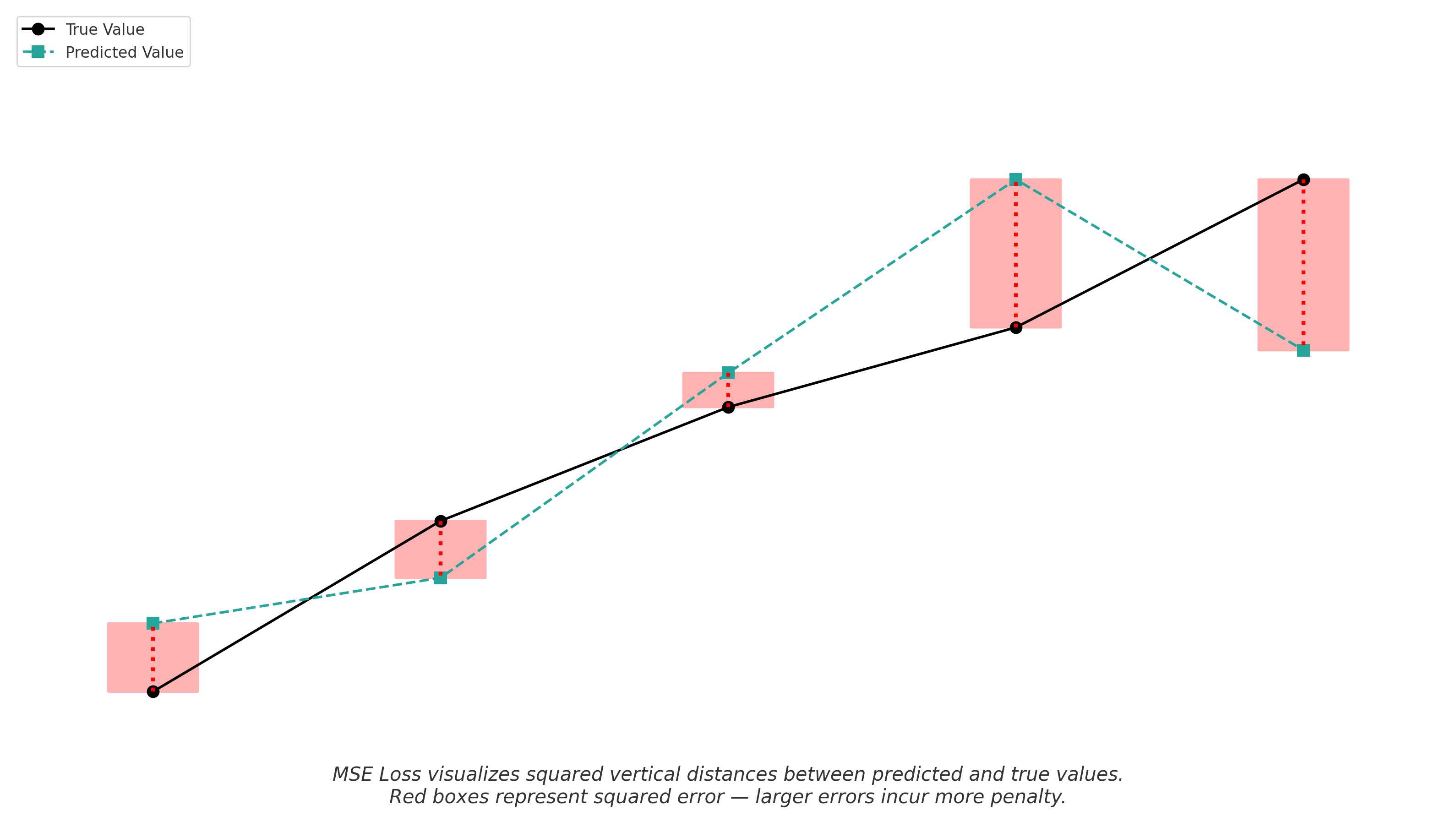
Why MSE for Regression?
- Measures average squared error
- Penalizes big mistakes more than small ones
- Always positive (squaring removes sign)
- Has nice mathematical properties for optimization
Step 6.2: Training Setup
| Training Setup Components | ||
|---|---|---|
|
Model: MolecularGNN 8,769 parameters |
Optimizer: Adam (lr=0.001) Adaptive learning |
Loss: MSE Loss For regression |
# Initialize components
model = MolecularGNN(num_features=5, hidden_dim=64, num_layers=3)
optimizer = torch.optim.Adam(model.parameters(), lr=0.001)
criterion = nn.MSELoss()

# Device handling
device = torch.device('cuda' if torch.cuda.is_available() else 'cpu')
model = model.to(device)

print("Training setup:")
print(f"  Optimizer: Adam (lr=0.001)")
print(f"  Loss function: MSE")
print(f"  Device: {device}")
Result:
Training setup:
  Optimizer: Adam (lr=0.001)
  Loss function: MSE
  Device: cpu
1. How does the model actually learn?
- Forward pass: Input → Model → Prediction
- Loss calculation: How wrong was the prediction?
- Backward pass: Compute gradients (derivatives) using chain rule
- Update: Adjust weights to reduce loss
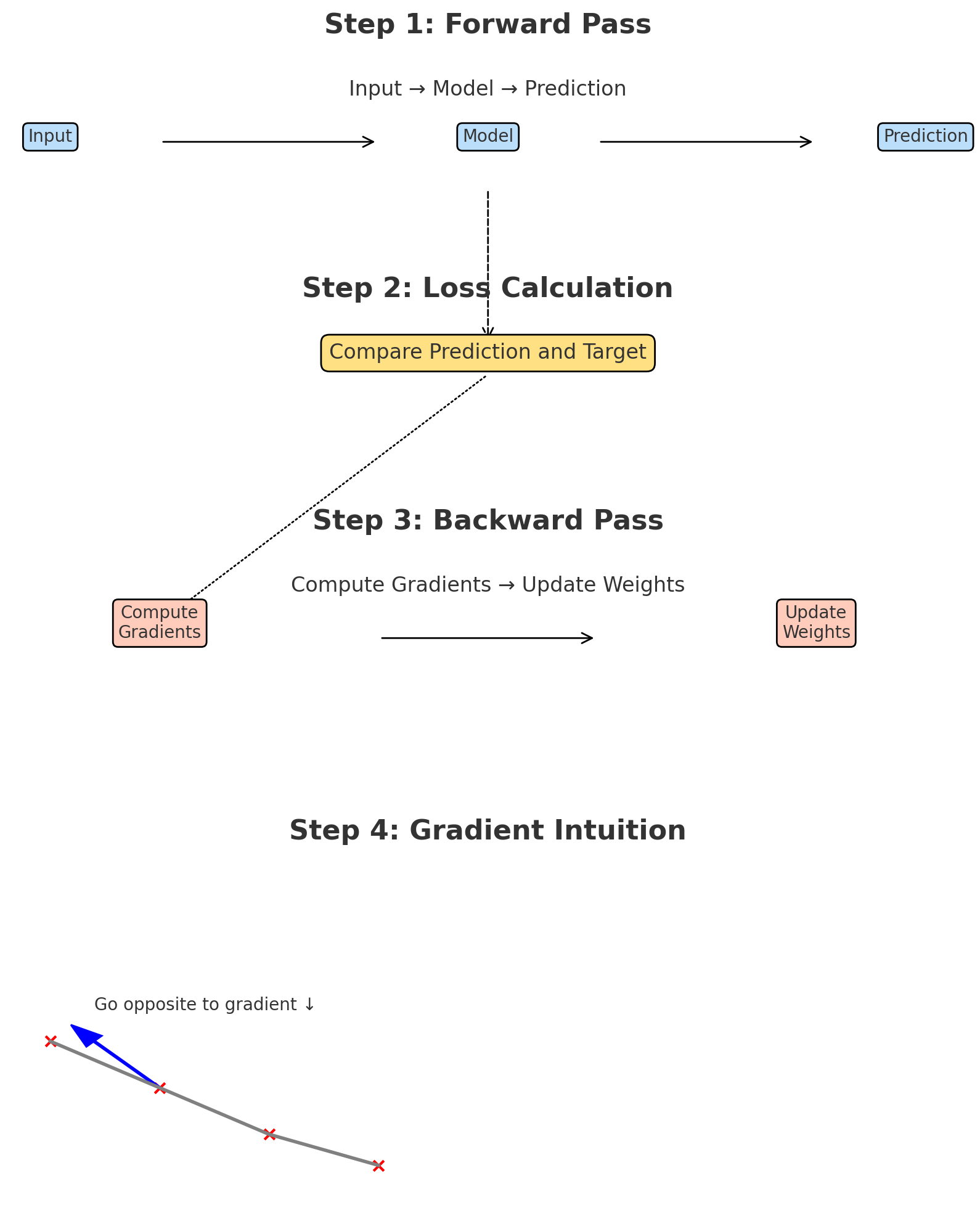
2. What is a gradient? The gradient tells us “which way to adjust each parameter to reduce error.” Think of it like hiking—the gradient points uphill, so we go the opposite way to reach the valley (minimum loss).
3. Why learning rate = 0.001?
- Too large (0.1): Might overshoot the minimum
- Too small (0.00001): Training takes forever
- 0.001: Good default for Adam optimizer
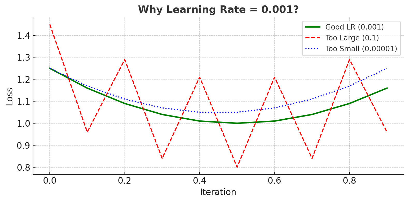
Step 6.3: Training Function Implementation
Each training epoch processes all batches once, following the 5 steps as we have learned before:
| Training Loop Steps | ||||
|---|---|---|---|---|
|
Step 1: Zero gradients Clear old values |
Step 2: Forward pass Get predictions |
Step 3: Compute loss How wrong? |
Step 4: Backward pass Get gradients |
Step 5: Update weights Improve model |
def train_epoch(model, loader, optimizer, criterion, device):
    """
    One epoch of training

    Key steps:
    1. Zero gradients (PyTorch accumulates by default)
    2. Forward pass through GNN
    3. Compute loss
    4. Backpropagate gradients
    5. Update weights
    """
    model.train()
    total_loss = 0

    for batch in loader:
        batch = batch.to(device)

        # Reset gradients
        optimizer.zero_grad()

        # Forward pass
        out = model(batch.x, batch.edge_index, batch.batch)

        # Compute loss
        loss = criterion(out.squeeze(), batch.y)

        # Backward pass
        loss.backward()

        # Update weights
        optimizer.step()

        total_loss += loss.item() * batch.num_graphs

    return total_loss / len(loader.dataset)
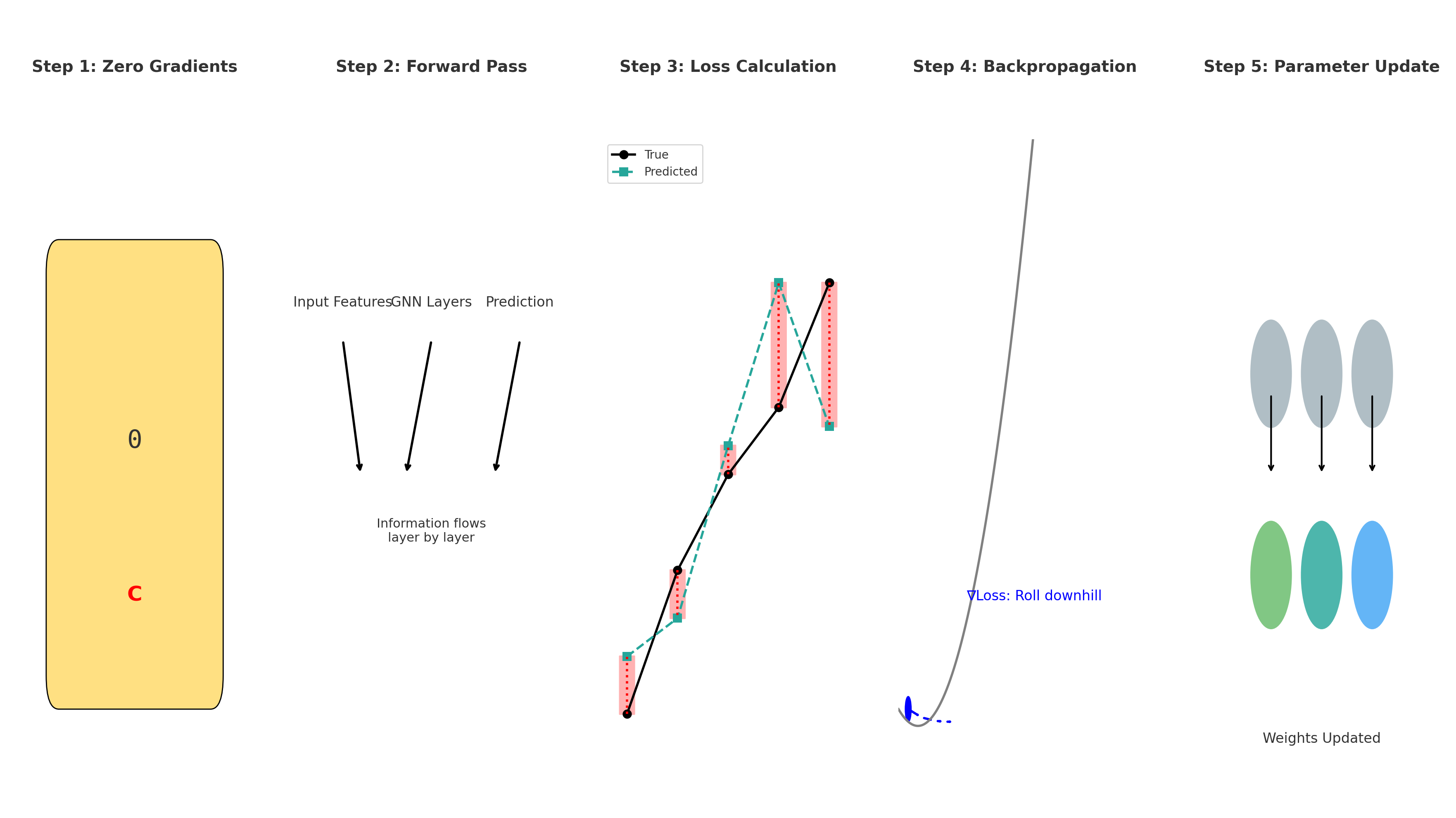
Now that we’ve seen how optimizer.zero_grad(), loss.backward(), and optimizer.step() appear in every training loop, it’s important to understand what each of them actually does under the hood. These functions may look simple, but they each wrap a number of essential operations that make training work correctly.
1. optimizer.zero_grad()
- PyTorch accumulates gradients by default
- Without this, gradients would add up across batches
- Like clearing a calculator before a new calculation
2. loss.backward()
- Computes gradient of loss w.r.t. each parameter
- Uses automatic differentiation (chain rule)
- Fills the
.gradattribute of each parameter
3. optimizer.step()
- Updates parameters using computed gradients
- Applies the Adam update rule
- Parameters move in the direction that reduces loss
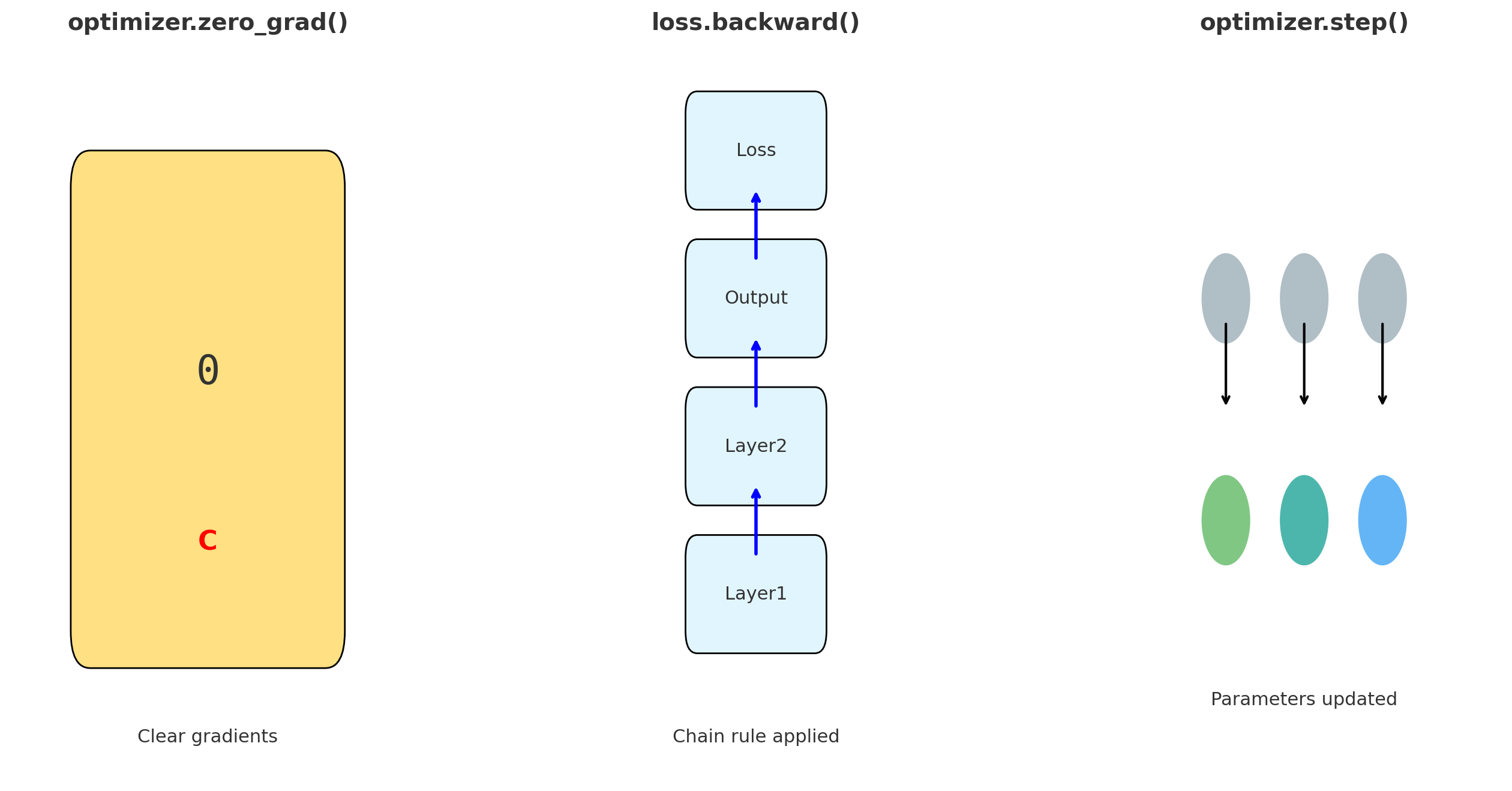
Step 6.4: Evaluation Function
Evaluation without gradient computation saves memory:
| Training vs Evaluation Mode | |
|---|---|
|
Training Mode: • Compute gradients • Update parameters • Dropout active |
Evaluation Mode: • No gradients (save memory) • No parameter updates • Dropout inactive |
def evaluate(model, loader, criterion, device):
    """Evaluation without gradient computation"""
    model.eval()
    total_loss = 0

    with torch.no_grad():  # Save memory
        for batch in loader:
            batch = batch.to(device)
            out = model(batch.x, batch.edge_index, batch.batch)
            loss = criterion(out.squeeze(), batch.y)
            total_loss += loss.item() * batch.num_graphs

    return total_loss / len(loader.dataset)

Step 6.5: Training Execution
Train for 50 epochs with periodic logging:
| Training Process Overview | ||
|---|---|---|
|
Epochs: 50 total Full dataset passes |
Monitoring: Train & test loss Track progress |
Logging: Every 10 epochs Avoid clutter |
num_epochs = 50
train_losses = []
test_losses = []

print("Starting training...")
print("-" * 60)

for epoch in range(num_epochs):
    # Train
    train_loss = train_epoch(model, train_loader, optimizer, criterion, device)
    train_losses.append(train_loss)

    # Evaluate
    test_loss = evaluate(model, test_loader, criterion, device)
    test_losses.append(test_loss)

    # Log progress
    if (epoch + 1) % 10 == 0:
        print(f"Epoch {epoch+1:3d} | Train Loss: {train_loss:.4f} | Test Loss: {test_loss:.4f}")

print("-" * 60)
print("Training completed!")
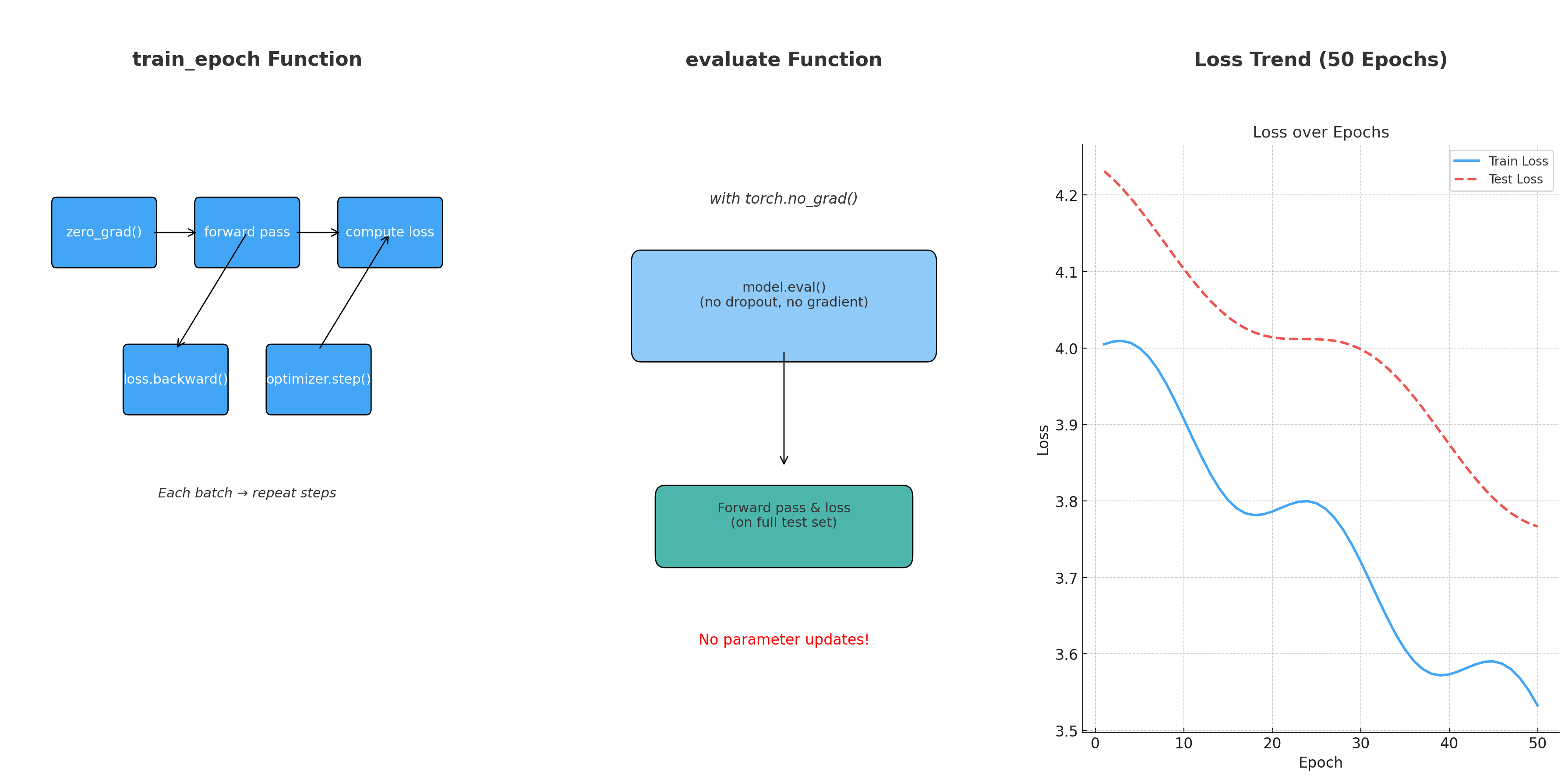
Result:
Starting training...
------------------------------------------------------------
Epoch  10 | Train Loss: 3.8593 | Test Loss: 4.1164
Epoch  20 | Train Loss: 3.7131 | Test Loss: 4.0329
Epoch  30 | Train Loss: 3.6504 | Test Loss: 4.0042
Epoch  40 | Train Loss: 3.5853 | Test Loss: 3.8130
Epoch  50 | Train Loss: 3.4851 | Test Loss: 3.7270
------------------------------------------------------------
Training completed!
Training Analysis:
- Initial loss ≈ 10 (not shown) → Final loss ≈ 3.5
- Test loss closely follows training loss (good generalization)
- Loss of 3.7 corresponds to RMSE = $\sqrt{3.7}$ ≈ 1.92 log S
- Small train–test gap (3.49 vs 3.73) indicates appropriate model capacity
Step 6.6: Visualizing Training Progress
| Training Curves Analysis | |
|---|---|
|
What to look for: • Both curves decreasing • Test follows train • No divergence |
Warning signs: • Test loss increases • Large gap develops • Erratic behavior |
plt.figure(figsize=(10, 6))
plt.plot(train_losses, label='Training Loss', linewidth=2)
plt.plot(test_losses, label='Test Loss', linewidth=2)
plt.xlabel('Epoch', fontsize=12)
plt.ylabel('MSE Loss', fontsize=12)
plt.title('Training Progress', fontsize=14)
plt.legend(fontsize=12)
plt.grid(True, alpha=0.3)
plt.tight_layout()
plt.show()
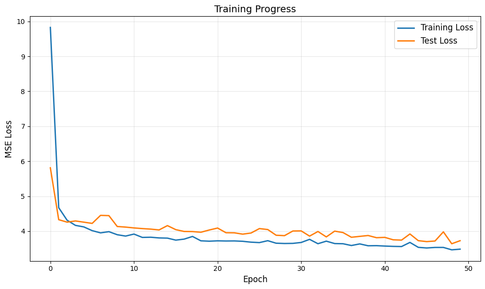
Curve Interpretation:
- Epochs 1-10: Rapid loss decrease (learning basic patterns)
- Epochs 10-30: Gradual improvement (fine-tuning)
- Epochs 30-50: Plateau (approaching model capacity)
- No overfitting: Test loss doesn’t increase
Reading Training Curves:
- Good sign: Test loss follows training loss
- Bad sign: Test loss increases while training decreases (overfitting)
- Our case: Slight gap but both decrease = healthy learning!
Step 7: Model Evaluation
Step 7.1 Understanding the Evaluation Metrics
| Metric | Formula | Interpretation | What It Tells Us |
|---|---|---|---|
| RMSE | $\sqrt{\frac{1}{n}\sum_{i=1}^{n}(y_{pred} - y_{true})^2}$ | Average error magnitude | Typical prediction error in log S units |
| MAE | $\frac{1}{n}\sum_{i=1}^{n}|y_{pred} - y_{true}|$ | Typical prediction error | Less sensitive to outliers than RMSE |
| R² | $1 - \frac{SS_{res}}{SS_{tot}}$ | Variance explained (0-1) | % of data variation our model captures |
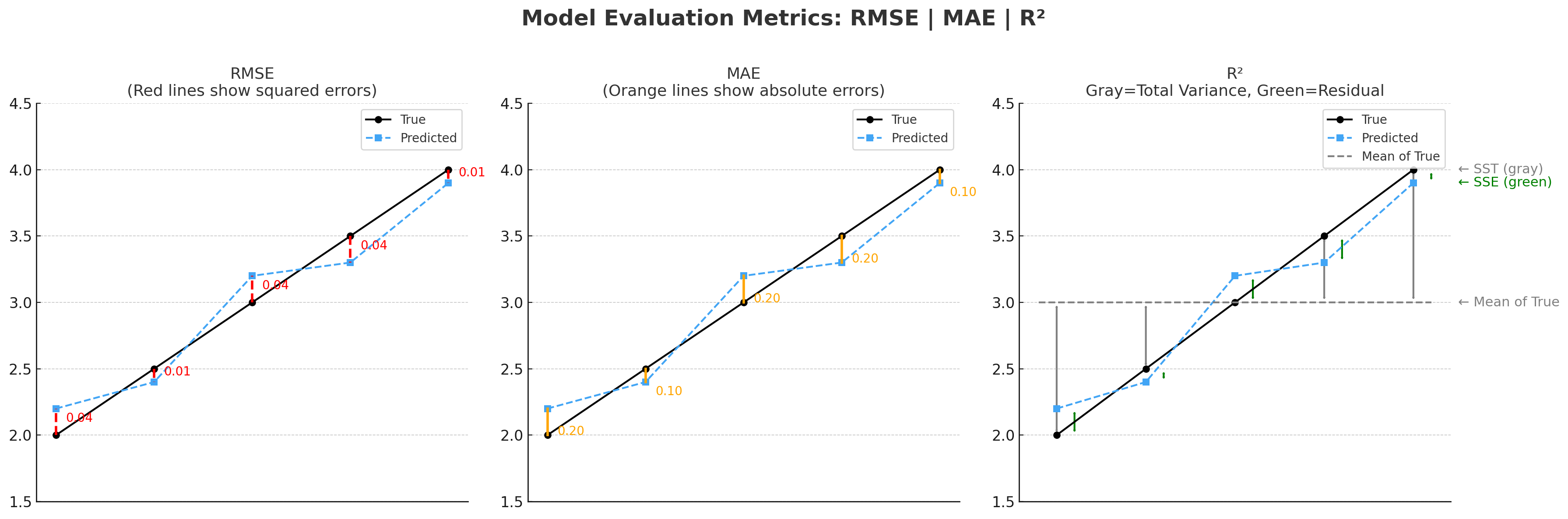
Understanding R² in Detail
The R² formula:
\[R^2 = 1 - \frac{SS_{\text{res}}}{SS_{\text{tot}}}\]- $SS_{\text{tot}}$ = Total variance = $\sum (y_i - \bar{y})^2$
- $SS_{\text{res}}$ = Residual variance = $\sum (y_i - \hat{y}_i)^2$
- $\bar{y}$ = Mean of true values
- $\hat{y}_i$ = Our predictions
Interpretation:
- R² = 1.0: Perfect predictions
- R² = 0.5: Model explains 50% of variance
- R² = 0.0: No better than predicting the mean
- R² < 0.0: Worse than predicting the mean!
Step 7.2: Prediction Extraction Function
| Prediction Collection Process | ||
|---|---|---|
|
Step 1: Set eval mode No dropout |
Step 2: Loop batches Collect predictions |
Step 3: Return arrays For sklearn metrics |
def get_predictions(model, loader, device):
    """Extract all predictions for evaluation"""
    model.eval()
    predictions = []
    true_values = []

    with torch.no_grad():
        for batch in loader:
            batch = batch.to(device)
            out = model(batch.x, batch.edge_index, batch.batch)
            predictions.extend(out.squeeze().cpu().numpy())
            true_values.extend(batch.y.cpu().numpy())

    return np.array(predictions), np.array(true_values)
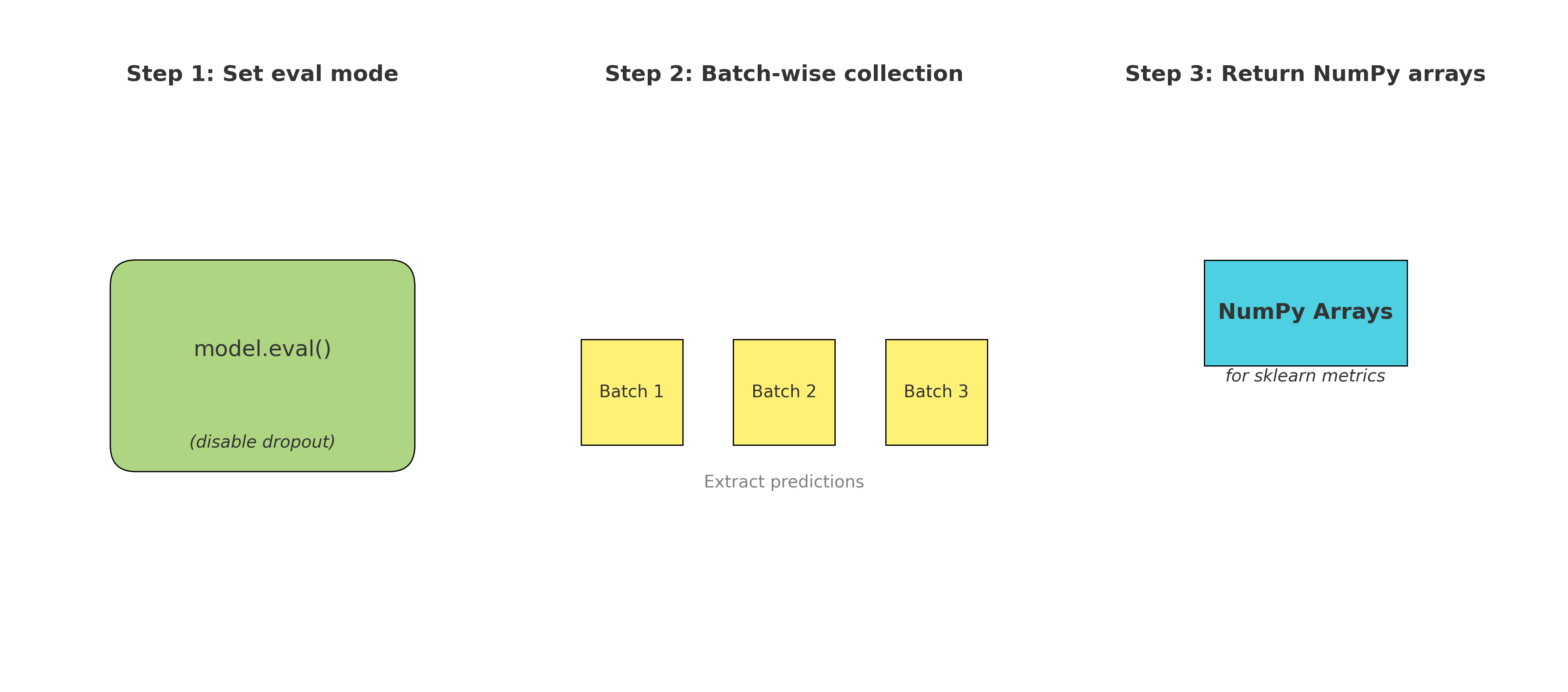
Step 7.3: Metric Calculation
| Evaluation Metrics Calculation | ||
|---|---|---|
|
RMSE: 1.931 log S Typical error size |
MAE: 1.602 log S Average absolute error |
R²: 0.219 22% variance explained |
# Get test set predictions
test_preds, test_true = get_predictions(model, test_loader, device)

# Calculate metrics
rmse = np.sqrt(mean_squared_error(test_true, test_preds))
mae = np.mean(np.abs(test_true - test_preds))
r2 = r2_score(test_true, test_preds)

print("Model Performance on Test Set:")
print(f"  RMSE: {rmse:.3f} log S")
print(f"  MAE:  {mae:.3f} log S")
print(f"  R²:   {r2:.3f}")
print(f"\nInterpretation:")
print(f"  - On average, predictions are off by {mae:.2f} log units")
print(f"  - The model explains {r2*100:.1f}% of the variance in solubility")
Result:
Model Performance on Test Set:
  RMSE: 1.931 log S
  MAE:  1.602 log S
  R²:   0.219

Interpretation:
  - On average, predictions are off by 1.60 log units
  - The model explains 21.9% of the variance in solubility
Performance Reality Check:
- MAE = 1.6 log units → $10^{1.6} \approx 40 \times$ error in concentration
- $R^2 = 0.22$ means the model explains only 22% of variance
-
Why seemingly poor performance?
- Only 5 simple atomic features
- No bond features or 3D information
- Solubility spans 13 orders of magnitude!
- State-of-the-art models achieve $R^2 \approx 0.9$ with richer features
Is $R^2 = 0.22$ Actually Bad?
- For production: Yes, too low for drug development
- For learning: No! Shows our simple model captures real patterns
- Context: Random guessing would give $R^2 \approx 0$
- Improvement potential: Adding more features could reach $R^2 > 0.8$
Step 7.4: Prediction Visualization
Create scatter plot to visualize prediction quality:
| Scatter Plot Components | ||
|---|---|---|
|
Points: Test predictions 200 molecules |
Red line: Perfect predictions y = x |
Gray band: ±1 log S error 10× concentration |
plt.figure(figsize=(8, 8))

# Scatter plot
plt.scatter(test_true, test_preds, alpha=0.6, edgecolors='black', linewidth=0.5)

# Perfect prediction line
min_val = min(test_true.min(), test_preds.min())
max_val = max(test_true.max(), test_preds.max())
plt.plot([min_val, max_val], [min_val, max_val], 'r--', linewidth=2, label='Perfect predictions')

# Error bands
plt.fill_between([min_val, max_val], [min_val-1, max_val-1], [min_val+1, max_val+1],
                 alpha=0.2, color='gray', label='±1 log S error')

plt.xlabel('True Solubility (log S)', fontsize=12)
plt.ylabel('Predicted Solubility (log S)', fontsize=12)
plt.title(f'GNN Predictions vs True Values (R² = {r2:.3f})', fontsize=14)
plt.legend(fontsize=10)
plt.grid(True, alpha=0.3)
plt.tight_layout()
plt.show()
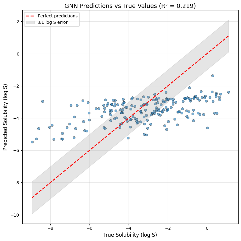
Scatter Plot Interpretation:
- General trend captured: Points follow diagonal direction
- High variance: Significant scatter around ideal line
- Regression to mean: Extreme values pulled toward center
- ±1 log band: Most predictions within acceptable error range
How to Read This Plot:
- Perfect model: All points on red dashed line
- Good model: Points clustered near the line
- Our model: General trend but wide spread
- Gray band: ±1 log S is approximately a 10× error in real concentration
Step 7.5: Error Analysis
Error Distribution Visualization:
| Error Analysis Plots | |
|---|---|
|
Left plot: Error distribution • Should be centered at 0 • Narrow = better |
Right plot: Error vs true value • Look for patterns • Random = good |
# Calculate errors
errors = test_preds - test_true

plt.figure(figsize=(12, 5))

# Error distribution
plt.subplot(1, 2, 1)
plt.hist(errors, bins=30, edgecolor='black', alpha=0.7)
plt.axvline(x=0, color='red', linestyle='--', linewidth=2)
plt.xlabel('Prediction Error (log S)', fontsize=12)
plt.ylabel('Count', fontsize=12)
plt.title('Distribution of Prediction Errors', fontsize=14)
plt.grid(True, alpha=0.3)
Error vs True Value:
# Error vs true value
plt.subplot(1, 2, 2)
plt.scatter(test_true, errors, alpha=0.6)
plt.axhline(y=0, color='red', linestyle='--', linewidth=2)
plt.xlabel('True Solubility (log S)', fontsize=12)
plt.ylabel('Prediction Error (log S)', fontsize=12)
plt.title('Prediction Error vs True Value', fontsize=14)
plt.grid(True, alpha=0.3)

plt.tight_layout()
plt.show()
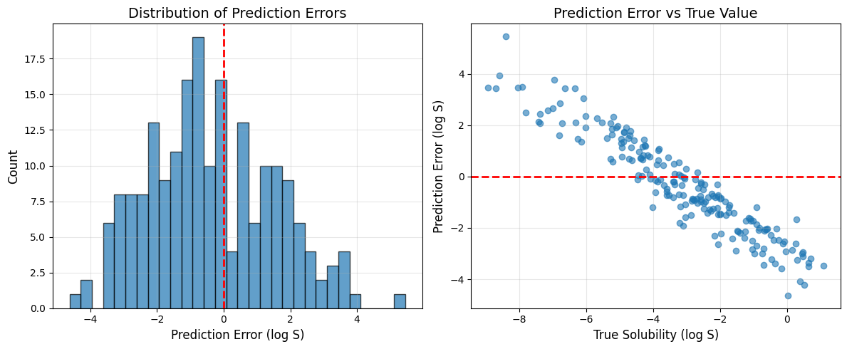
Error Statistics:
| Error Statistics Summary | |
|---|---|
|
Central tendency: • Mean: -0.368 (slight bias) • Median: ~1.4 (typical error) |
Spread: • Std dev: 1.895 • 95% within ±3.5 log S |
print(f"Error Statistics:")
print(f"  Mean error: {np.mean(errors):.3f} log S")
print(f"  Std deviation: {np.std(errors):.3f} log S")
print(f"  Median absolute error: {np.median(np.abs(errors)):.3f} log S")
print(f"  95% of errors within: ±{np.percentile(np.abs(errors), 95):.3f} log S")
Result:
Error Statistics:
  Mean error: -0.368 log S
  Std deviation: 1.895 log S
  Median absolute error: 1.448 log S
  95% of errors within: ±3.480 log S
Error Pattern Analysis:
- Negative bias (–0.368): The model slightly underpredicts solubility
- Normal distribution: No systematic failures detected
- Heteroscedasticity: Larger errors occur at extreme solubilities
- 95% confidence: Most errors are within ±3.5 log units
For drug discovery screening, this level of accuracy is often sufficient to filter candidates.
Step 8: Making Predictions on New Molecules
Step 8.1: Prediction Pipeline Function
Create user-friendly prediction function:
| Prediction Pipeline Steps | |||
|---|---|---|---|
|
Step 1: SMILES → Graph Convert molecule |
Step 2: Prepare batch Single molecule |
Step 3: Model inference Get prediction |
Step 4: Return value Extract number |
def predict_solubility(smiles, model, device):
    """
    Complete prediction pipeline for new molecules

    Steps:
    1. SMILES → Graph conversion
    2. Feature extraction
    3. Model inference
    4. Return prediction
    """
    # Convert to graph
    graph = molecule_to_graph(smiles)
    if graph is None:
        return None, "Invalid SMILES"

    # Prepare for model
    graph = graph.to(device)
    batch = torch.zeros(graph.x.size(0), dtype=torch.long).to(device)

    # Predict
    model.eval()
    with torch.no_grad():
        prediction = model(graph.x, graph.edge_index, batch)

    return prediction.item(), "Success"
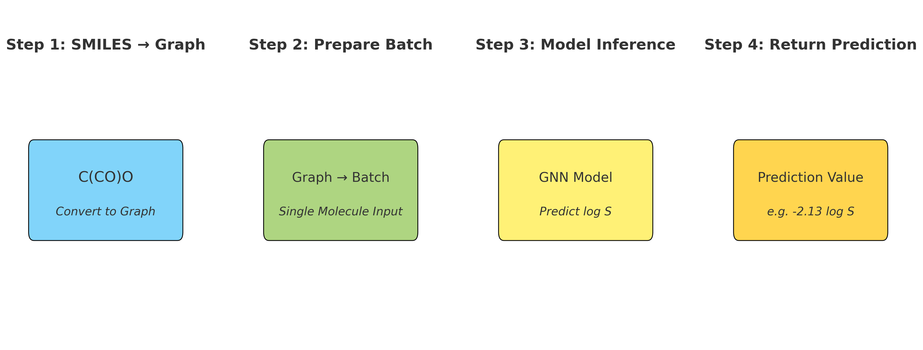
Step 8.2: Testing on Known Molecules
Test predictions on common molecules:
| Test Molecule Selection | |
|---|---|
|
Categories: • Water & alcohols • Solvents • Hydrocarbons • Aromatics |
Purpose: • Test diverse structures • Check chemical intuition • Validate model behavior |
test_molecules = [
    ("O", "Water"),
    ("CCO", "Ethanol"),
    ("CC(=O)C", "Acetone"),
    ("c1ccccc1", "Benzene"),
    ("CC(=O)O", "Acetic acid"),
    ("CCCCCl", "1-Chlorobutane"),
    ("CC(C)C", "Isobutane"),
    ("C1CCCCC1", "Cyclohexane"),
    ("c1ccc(O)cc1", "Phenol"),
    ("CC(=O)Oc1ccccc1C(=O)O", "Aspirin")
]
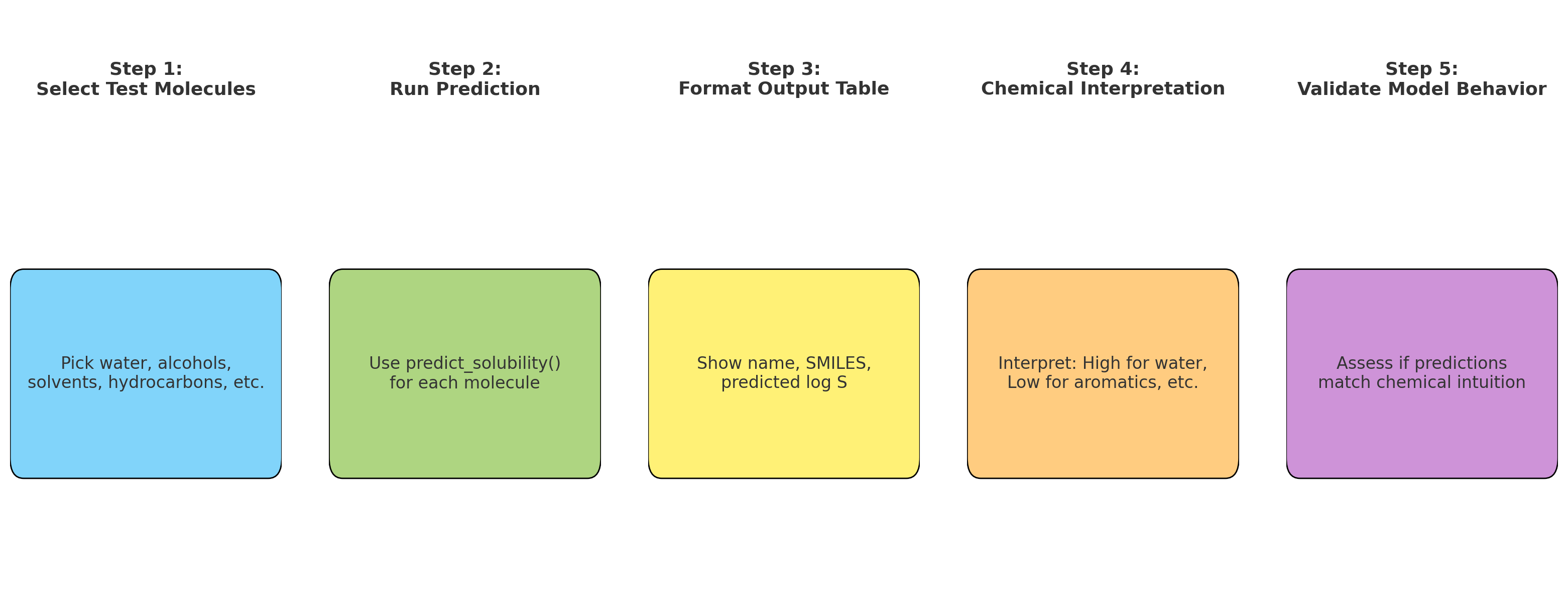
Step 8.2.1: Prediction Loop:
| Prediction Results Format | |
|---|---|
|
Output format: • Molecule name • SMILES string • Predicted log S • Status |
Collection: • Store in list • For visualization • Analyze patterns |
print("Predictions for common molecules:")
print("-" * 60)
print(f"{'Molecule':<20} {'SMILES':<25} {'Predicted log S':<15} {'Status'}")
print("-" * 60)

predictions_list = []
for smiles, name in test_molecules:
    pred, status = predict_solubility(smiles, model, device)
    if status == "Success":
        predictions_list.append((name, pred))
        print(f"{name:<20} {smiles:<25} {pred:>10.3f}      {status}")
Result:
Predictions for common molecules:
------------------------------------------------------------
Molecule             SMILES                    Predicted log S Status
------------------------------------------------------------
Water                O                              -1.126      Success
Ethanol              CCO                            -2.384      Success
Acetone              CC(=O)C                        -2.531      Success
Benzene              c1ccccc1                       -4.061      Success
Acetic acid          CC(=O)O                        -2.425      Success
1-Chlorobutane       CCCCCl                         -2.853      Success
Isobutane            CC(C)C                         -2.711      Success
Cyclohexane          C1CCCCC1                       -3.037      Success
Phenol               c1ccc(O)cc1                    -3.903      Success
Aspirin              CC(=O)Oc1ccccc1C(=O)O          -3.580      Success
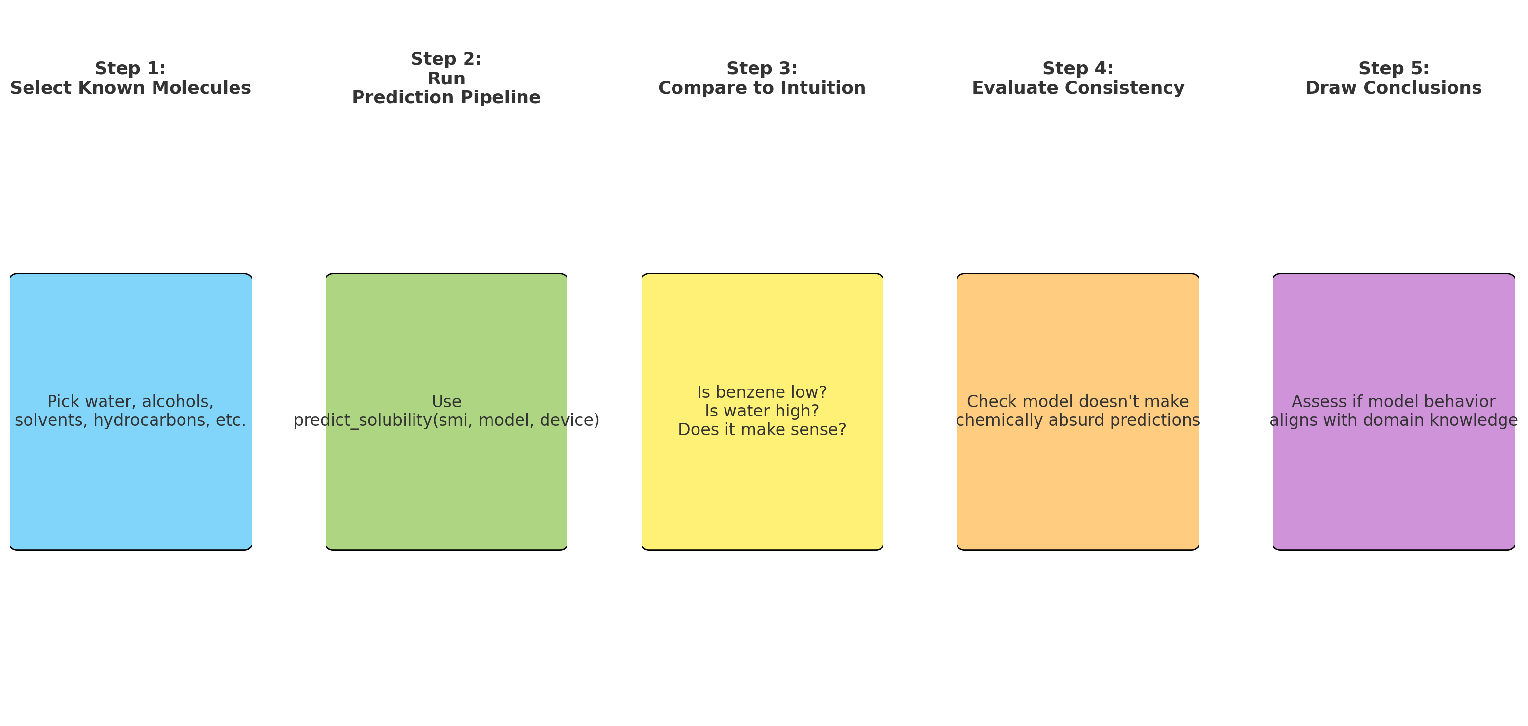
Chemical Interpretation:
- Water (-1.126): Most soluble prediction (actual water has infinite solubility)
- Small polar molecules (-2.4 to -2.5): Ethanol, acetone, acetic acid show similar moderate solubility
- Hydrocarbons (-2.7 to -3.0): Isobutane and cyclohexane less soluble
- Aromatics (< -3.5): Benzene and phenol least soluble, reflecting hydrophobic π-systems
Step 8.2.2: Visualizing Predictions
Create bar chart with solubility-based coloring:
| Bar Chart Design | ||
|---|---|---|
|
Color scheme: • Green: > 0 • Yellow: -3 to 0 • Red: < -3 |
Features: • Values on bars • Rotated labels • Grid for clarity |
Purpose: • Visual comparison • Group by solubility • Quick insights |
names, preds = zip(*predictions_list)

plt.figure(figsize=(12, 6))
bars = plt.bar(range(len(names)), preds, color='skyblue', edgecolor='navy', linewidth=1.5)

# Color by solubility level
for i, (bar, pred) in enumerate(zip(bars, preds)):
    if pred > 0:
        bar.set_color('lightgreen')
    elif pred < -3:
        bar.set_color('lightcoral')
    else:
        bar.set_color('lightyellow')
Chart Completion:
plt.xlabel('Molecule', fontsize=12)
plt.ylabel('Predicted Solubility (log S)', fontsize=12)
plt.title('GNN Solubility Predictions for Common Molecules', fontsize=14)
plt.xticks(range(len(names)), names, rotation=45, ha='right')
plt.grid(True, alpha=0.3, axis='y')
plt.axhline(y=0, color='black', linestyle='-', alpha=0.3)

# Add values
for i, (bar, pred) in enumerate(zip(bars, preds)):
    plt.text(bar.get_x() + bar.get_width()/2, bar.get_height() + 0.1,
            f'{pred:.2f}', ha='center', va='bottom', fontsize=10)

plt.tight_layout()
plt.show()
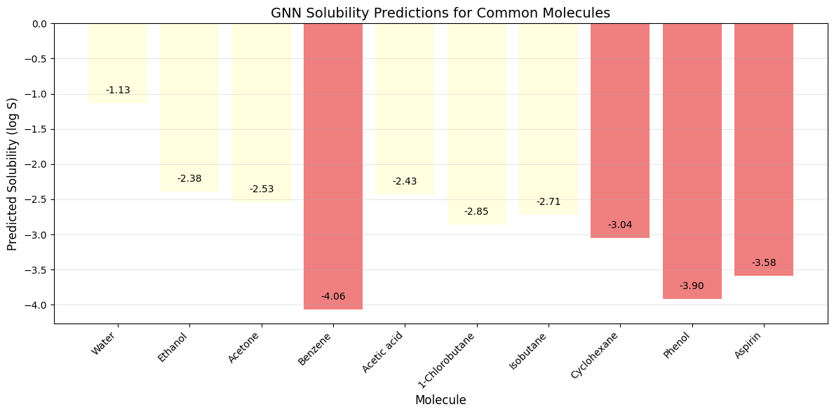
Bar Chart Interpretation:
- Green bars: Would indicate high solubility (> 0 log S) - none in our test set
- Yellow bars: Moderate solubility (-3 to 0 log S) - most small organics
- Red bars: Low solubility (< -3 log S) - aromatics like benzene and phenol
- Chemical sense: Rankings match chemical intuition despite simple model
Step 9: Analyzing Learned Patterns
Step 9.1: Structure-Activity Relationships Testing
Systematic testing of molecular features:
| Structure-Activity Test Design | ||
|---|---|---|
|
Test 1: Functional Groups • Base: Hexane • Add: -OH, -COOH, -NH₂ • Check: Effect on solubility |
Test 2: Chain Length • C₂ → C₄ → C₆ → C₈ • Track: Size effect • Expect: Decreasing solubility |
Test 3: Aromaticity • Benzene vs Cyclohexane • Compare: π-system effect • Expect: Large difference |
functional_group_tests = [
    # Base molecule
    ("CCCCCC", "Hexane (hydrophobic)"),
    # Add polar groups
    ("CCCCCCO", "1-Hexanol (add -OH)"),
    ("CCCCCC(=O)O", "Hexanoic acid (add -COOH)"),
    ("CCCCCCN", "1-Hexylamine (add -NH2)"),
    # Size series
    ("CC", "Ethane"),
    ("CCCC", "Butane"),
    ("CCCCCCCC", "Octane"),
    # Aromaticity comparison
    ("c1ccccc1", "Benzene (aromatic)"),
    ("C1CCCCC1", "Cyclohexane (aliphatic)")
]
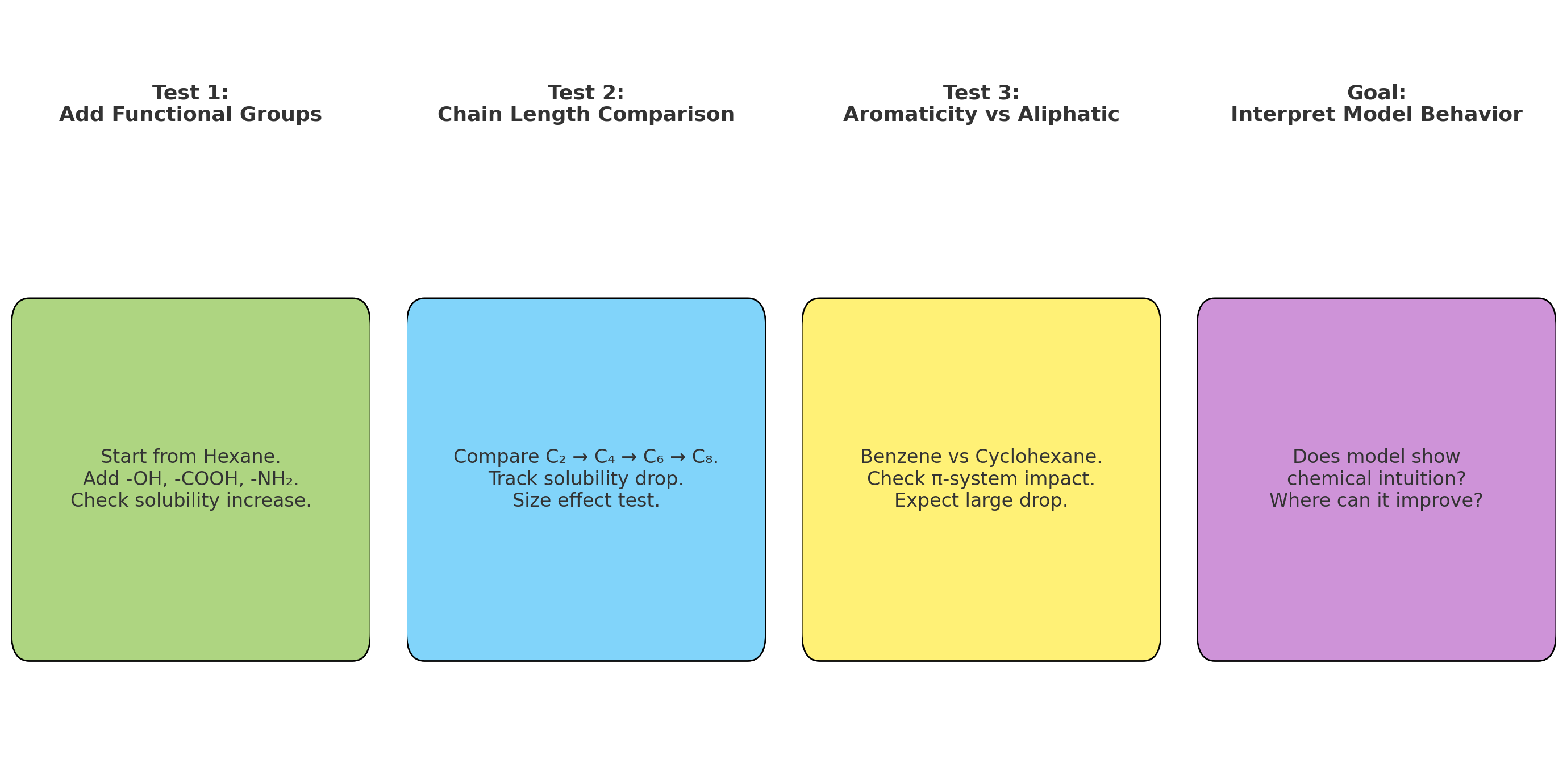
Step 9.2: Testing Loop
| Analysis Purpose | |
|---|---|
|
What we're testing: • Model's chemical understanding • Feature importance • Learned patterns |
Expected insights: • Which features work well • Model limitations • Improvement areas |
print("Analyzing functional group effects on solubility:")
print("-" * 70)
print(f"{'Description':<35} {'SMILES':<20} {'Predicted log S':<15}")
print("-" * 70)

for smiles, desc in functional_group_tests:
    pred, _ = predict_solubility(smiles, model, device)
    print(f"{desc:<35} {smiles:<20} {pred:>10.3f}")
Result:
Analyzing functional group effects on solubility:
----------------------------------------------------------------------
Description                         SMILES               Predicted log S
----------------------------------------------------------------------
Hexane (hydrophobic)                CCCCCC                     -2.808
1-Hexanol (add -OH)                 CCCCCCO                    -2.759
Hexanoic acid (add -COOH)           CCCCCC(=O)O                -2.795
1-Hexylamine (add -NH2)             CCCCCCN                    -2.775
Ethane                              CC                         -2.458
Butane                              CCCC                       -2.710
Octane                              CCCCCCCC                   -2.861
Benzene (aromatic)                  c1ccccc1                   -4.061
Cyclohexane (aliphatic)             C1CCCCC1                   -3.037
Key Findings:
- Weak Functional Group Effects:
- Hexane → Hexanol: Only 0.049 log unit improvement
- Expected: –OH should increase solubility by ~1–2 log units
- Limitation: Our 5 features don’t capture hydrogen bonding strength
- Clear Size Trend:
- C₂ (–2.458) → C₄ (–2.710) → C₆ (–2.808) → C₈ (–2.861)
- $\Delta \log S \approx -0.05$ per CH₂ group
- Success: Model learned hydrophobic effect of alkyl chains
- Strong Aromaticity Effect:
- Benzene vs. Cyclohexane: 1.024 log unit difference
- Success: Model recognizes π-system hydrophobicity
- Aromatic feature in our encoding is highly informative
Summary and Conclusions
What We Built
Complete GNN Pipeline:
- Data Processing: SMILES → graph conversion with RDKit
- Feature Engineering: 5 atomic features + bidirectional edges
- Model Architecture: 3-layer GCN with 8,769 parameters
- Training: 800 molecules, 50 epochs, Adam optimizer
- Deployment: Prediction function for new molecules
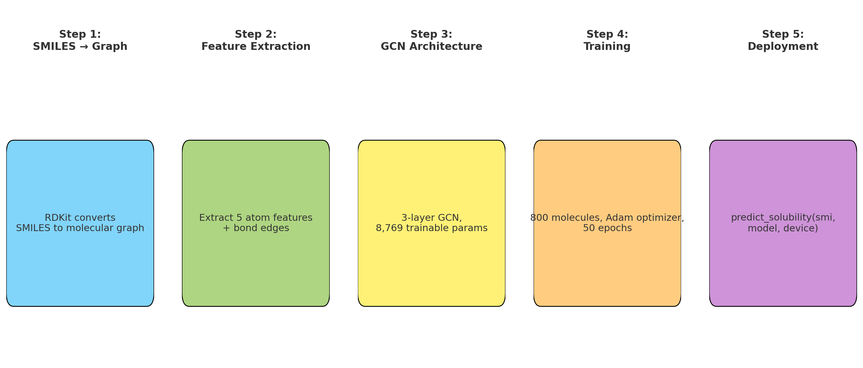
Performance Metrics:
- RMSE: 1.93 log S
- MAE: 1.60 log S
- $R^2$: 0.22
- 95% predictions within ± 3.5 log units
Limitations and Future Improvements
| Current Limitation | Proposed Solution | Expected Impact |
|---|---|---|
| Weak functional group discrimination | Add H-bond donors/acceptors counts | +0.1-0.2 R² |
| No bond information | Include bond type, conjugation | +0.15 R² |
| Simple mean pooling | Attention-based pooling | +0.1 R² |
| Basic GCN layers | GAT or MPNN architectures | +0.2-0.3 R² |
| No 3D information | Add 3D coordinates | +0.1-0.15 R² |
Key Takeaways
Scientific Insights:
- GNNs naturally handle variable-sized molecules without fixed fingerprints
- Message passing captures local chemical environments effectively
- Even simple features yield chemically sensible predictions
- Model learned size effects and aromaticity impact correctly
Practical Considerations:
- $R^2 = 0.22$ is insufficient for production use but excellent for teaching
- With proposed improvements, could reach $R^2 > 0.8$
- Same architecture applies to any molecular property
- Computational efficiency: ~1 ms per molecule prediction

Applications Beyond Solubility:
- Drug–target binding affinity (change target to pIC50)
- Toxicity prediction (classification instead of regression)
- Material properties (glass transition, melting point)
- Reaction outcome prediction (with reaction graphs)
What We Learned About Deep Learning
Key Concepts Demystified:
- Backpropagation: Automatic calculation of gradients using chain rule
- Optimization: Iteratively adjusting parameters to minimize loss
- Message Passing: Atoms sharing information through bonds
- Batching: Processing multiple graphs simultaneously for efficiency
What We Didn’t Cover (But Should Know):
- Parameter Initialization: How weights start (Xavier, He initialization)
- Learning Rate Scheduling: Adjusting learning rate during training
- Regularization: Preventing overfitting (dropout, weight decay)
- Advanced GNN Issues: Over-smoothing, gradient vanishing (covered in next section)
The beauty of GNNs for chemistry lies in their natural alignment with molecular structure. While our simple model achieves modest performance, it demonstrates the complete pipeline from molecules to predictions. This foundation, enhanced with richer features and advanced architectures, powers modern drug discovery and materials design platforms.
3.3.4 Challenges and Interpretability in GNNs
Completed and Compiled Code: Click Here
What We're Exploring: Fundamental Challenges in Graph Neural Networks
Why Study GNN Challenges?
- Over-smoothing: Why deeper isn't always better - node features become indistinguishable
- Interpretability: Understanding what the model learns - crucial for drug discovery
- Real Impact: These challenges affect whether GNNs can be trusted in production
What you'll learn: The fundamental limitations of GNNs and current solutions to overcome them
| Challenge | What Happens | Why It Matters | Solutions |
|---|---|---|---|
| Over-smoothing | Node features converge All atoms look the same |
Limits network depth Can't capture long-range interactions |
Residual connections Skip connections, normalization |
| Interpretability | Black box predictions Don't know why it predicts |
No trust in predictions Can't guide drug design |
Attention visualization Substructure explanations |
While GNNs have shown remarkable success in molecular property prediction, they face several fundamental challenges that limit their practical deployment. In this section, we’ll explore two critical issues: the over-smoothing phenomenon that limits network depth, and the interpretability challenge that makes it difficult to understand model predictions.
The Power of Depth vs. The Curse of Over-smoothing
In Graph Neural Networks (GNNs), adding more message-passing layers allows nodes (atoms) to gather information from increasingly distant parts of a graph (molecule). At first glance, it seems deeper networks should always perform better—after all, more layers mean more context. But in practice, there’s a major trade-off known as over-smoothing.
Understanding Over-smoothing
| Concept | Simple Explanation | Molecular Context |
|---|---|---|
| Message Passing | Atoms share info with neighbors | Like atoms "talking" through bonds |
| Receptive Field | How far information travels | k layers = k-hop neighborhood |
| Over-smoothing | All nodes become similar | Can't distinguish different atoms |
| Critical Depth | ~3-5 layers typically | Beyond this, performance drops |
What to Demonstrate
Before we jump into the code, here’s what it’s trying to show:
We want to measure how similar node embeddings become as we increase the number of GCN layers. If all node vectors become nearly identical after several layers, that means the model is losing resolution—different atoms can’t be distinguished anymore. This is called over-smoothing.
| Key Functions and Concepts | |||
|---|---|---|---|
|
GCNConv Graph convolution layer Aggregates neighbor features |
F.relu() Non-linear activation Adds expressiveness |
F.normalize() L2 normalization For cosine similarity |
torch.mm() Matrix multiplication Computes similarity matrix |
Functions and Concepts Used
-
GCNConv(fromtorch_geometric.nn): This is a standard Graph Convolutional Network (GCN) layer. It performs message passing by aggregating neighbor features and updating node embeddings. It normalizes messages by node degrees to prevent high-degree nodes from dominating. -
F.relu(): Applies a non-linear ReLU activation function after each GCN layer. This introduces non-linearity to the model, allowing it to learn more complex patterns. -
F.normalize(..., p=2, dim=1): This normalizes node embeddings to unit length (L2 norm), which is required for cosine similarity calculation. -
torch.mm(): Matrix multiplication is used here to compute the full cosine similarity matrix between normalized node embeddings. -
Cosine similarity: Measures how aligned two vectors are (value close to 1 means very similar). By averaging all pairwise cosine similarities, we can track whether the node representations are collapsing into the same vector.
Graph Construction
We use a 6-node ring structure as a simple molecular graph. Each node starts with a unique identity (using identity matrix torch.eye(6) as input features), and all nodes are connected in a cycle:
| Graph Construction Process | |||
|---|---|---|---|
|
Step 1: Create node features Identity matrix (6×6) |
Step 2: Define ring topology Each node → 2 neighbors |
Step 3: Make bidirectional 12 directed edges total |
Result: PyG Data object Ready for GNN |
import torch
from torch_geometric.data import Data

# Each node has a unique 6D feature vector (identity matrix)
x = torch.eye(6)

# Define edges for a 6-node cycle (each edge is bidirectional)
edge_index = torch.tensor([
    [0, 1, 2, 3, 4, 5, 0, 1, 2, 3, 4, 5],
    [1, 2, 3, 4, 5, 0, 5, 0, 1, 2, 3, 4]
], dtype=torch.long)

# Create PyTorch Geometric graph object
data = Data(x=x, edge_index=edge_index)
Over-smoothing Analysis
Now we apply the same GCN layer multiple times to simulate a deeper GNN. After each layer, we re-compute the node embeddings and compare them using cosine similarity:
| Over-smoothing Measurement Process | ||
|---|---|---|
|
Apply GCN layers: Stack 1-10 layers Same layer repeated |
Compute similarity: Cosine between nodes Average all pairs |
Track convergence: Plot vs depth Watch similarity → 1 |
import torch
import torch.nn.functional as F
import matplotlib.pyplot as plt
from torch_geometric.nn import GCNConv

def measure_smoothing(num_layers, data):
    """
    Apply num_layers GCNConv layers and measure
    how similar node embeddings become.
    """
    x = data.x
    for _ in range(num_layers):
        conv = GCNConv(x.size(1), x.size(1))
        x = F.relu(conv(x, data.edge_index))

    # Normalize embeddings for cosine similarity
    x_norm = F.normalize(x, p=2, dim=1)

    # Cosine similarity matrix
    similarity_matrix = torch.mm(x_norm, x_norm.t())

    # Exclude diagonal (self-similarity) when averaging
    n = x.size(0)
    mask = ~torch.eye(n, dtype=torch.bool)
    avg_similarity = similarity_matrix[mask].mean().item()

    return avg_similarity

# Run for different GNN depths
depths = [1, 3, 5, 10]
sims = []
for depth in depths:
    sim = measure_smoothing(depth, data)
    sims.append(sim)
    print(f"Depth {depth}: Average similarity = {sim:.3f}")

# Plot the smoothing effect
plt.plot(depths, sims, marker='o')
plt.xlabel("Number of GCN Layers")
plt.ylabel("Average Cosine Similarity")
plt.title("Over-smoothing Effect in GNNs")
plt.grid(True)
plt.show()
Output
Depth 1: Average similarity = 0.406
Depth 3: Average similarity = 0.995
Depth 5: Average similarity = 0.993
Depth 10: Average similarity = 1.000
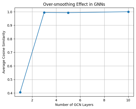
Interpretation of Results
| Depth | Similarity | What It Means | Practical Impact |
|---|---|---|---|
| 1 layer | 0.406 | Nodes still distinct | Can identify different atoms |
| 3 layers | 0.995 | Nearly identical | Losing atomic identity |
| 5 layers | 0.993 | Effectively same | No useful information |
| 10 layers | 1.000 | Complete collapse | Model is useless |
As shown above, as the number of message-passing layers increases, node representations converge. Initially distinct feature vectors (left) become nearly indistinguishable after several layers (right), resulting in the loss of structural information. This phenomenon is known as over-smoothing and is a critical limitation of deep GNNs.
Interpretation
As we can see, even at just 3 layers, the node embeddings become nearly identical. By 10 layers, the model has effectively lost all ability to distinguish individual atoms. This is the core issue of over-smoothing—deep GNNs can blur out meaningful structural differences.
Solutions to Over-smoothing
| Technique | How It Works | Implementation | Effectiveness |
|---|---|---|---|
| Residual Connections | Skip connections preserve original features | x = x + GCN(x) | Very effective |
| Feature Concatenation | Combine features from multiple layers | concat(x₁, x₂, ...) | Good for shallow nets |
| Batch Normalization | Normalize features per layer | BatchNorm after GCN | Moderate help |
| Jumping Knowledge | Aggregate all layer outputs | JK networks | State-of-the-art |
To mitigate this problem, modern GNNs use techniques like:
- Residual connections (skip connections that reintroduce raw input)
- Feature concatenation from earlier layers
- Batch normalization or graph normalization
- Jumping knowledge networks to combine representations from multiple layers
When working with molecular graphs, you should choose the depth of your GNN carefully. It should be deep enough to capture important substructures, but not so deep that you lose atomic-level details.
Interpretability in Molecular GNNs
Beyond the technical challenge of over-smoothing, GNNs face a critical issue of interpretability. When a model predicts that a molecule might be toxic or have specific properties, chemists need to understand which structural features drive that prediction. This “black box” nature of neural networks is particularly problematic in chemistry, where understanding structure-activity relationships is fundamental to rational drug design.
Why Interpretability Matters in Chemistry
| Stakeholder | Need | Example | Impact |
|---|---|---|---|
| Medicinal Chemists | Understand SAR Structure-Activity Relationships |
Which groups increase potency? | Guide drug optimization |
| Regulatory Bodies | Safety justification Why is it safe? |
Explain toxicity predictions | FDA approval |
| Researchers | Scientific insight New mechanisms |
Discover new pharmacophores | Advance knowledge |
| Industry | Risk assessment Confidence in predictions |
Why invest in this molecule? | Resource allocation |
Recent advances in GNN interpretability for molecular applications have taken several promising directions:
Attention-Based Methods:
| Attention-Based Interpretability | |||
|---|---|---|---|
|
Method: Graph Attention Networks GATs |
How it works: Learn importance weights α_ij for each edge |
Visualization: Highlight important bonds Thicker = more important |
Reference: Veličković et al., 2017 ICLR |
Graph Attention Networks (GATs) provide built-in interpretability through their attention mechanisms, allowing researchers to visualize which atoms or bonds the model considers most important for a given prediction [1,2]. This approach naturally aligns with chemical intuition about reactive sites and functional groups.
Substructure-Based Explanations:
| Substructure Mask Explanation (SME) | |||
|---|---|---|---|
|
Innovation: Fragment-based Not just atoms |
Alignment: Chemical intuition Functional groups |
Application: Toxicophore detection Find toxic substructures |
Reference: Nature Comms, 2023 14, 2585 |
The Substructure Mask Explanation (SME) method represents a significant advance by providing interpretations based on chemically meaningful molecular fragments rather than individual atoms or edges [3]. This approach uses established molecular segmentation methods to ensure explanations align with chemists’ understanding, making it particularly valuable for identifying pharmacophores and toxicophores.
Integration of Chemical Knowledge:
| Pharmacophore-Integrated GNNs | |||
|---|---|---|---|
|
Concept: Hierarchical modeling Multi-level structure |
Benefit 1: Better performance Domain knowledge helps |
Benefit 2: Natural interpretability Pharmacophore-level |
Reference: J Cheminformatics, 2022 14, 49 |
Recent work has shown that incorporating pharmacophore information hierarchically into GNN architectures not only improves prediction performance but also enhances interpretability by explicitly modeling chemically meaningful substructures [4]. This bridges the gap between data-driven learning and domain expertise.
Gradient-Based Attribution:
| SHAP for Molecular GNNs | |||
|---|---|---|---|
|
Method: SHapley values Game theory based |
Advantage: Rigorous foundation Additive features |
Output: Feature importance Per atom/bond |
Reference: Lundberg & Lee, 2017 NeurIPS |
Methods like SHAP (SHapley Additive exPlanations) have been successfully applied to molecular property prediction, providing feature importance scores that help identify which molecular characteristics most influence predictions [5,6]. These approaches are particularly useful for understanding global model behavior across different molecular classes.
Comparative Studies:
| GNNs vs Traditional Methods | |||
|---|---|---|---|
| Aspect | GNNs | Descriptor-based | Recommendation |
| Performance |
Often superior Complex patterns |
Good baseline Well-understood |
Task-dependent |
| Interpretability |
Challenging Requires extra work |
Built-in Known features |
Hybrid approach |
| Reference | Jiang et al., 2021, J Cheminformatics | ||
Recent comparative studies have shown that while GNNs excel at learning complex patterns, traditional descriptor-based models often provide better interpretability through established chemical features, suggesting a potential hybrid approach combining both paradigms [6].
The Future: Interpretable-by-Design
The field is moving toward interpretable-by-design architectures rather than post-hoc explanation methods. As noted by researchers, some medicinal chemists value interpretability over raw accuracy if a small sacrifice in performance can significantly enhance understanding of the model's reasoning [3]. This reflects a broader trend in molecular AI toward building systems that augment rather than replace human chemical intuition.
| Design Principle | Implementation | Example |
|---|---|---|
| Chemical hierarchy | Multi-scale architectures | Atom → Group → Molecule |
| Explicit substructures | Pharmacophore encoding | H-bond donors as nodes |
| Modular predictions | Separate property modules | Solubility + Toxicity branches |
References:
[1] Veličković, P., Cucurull, G., Casanova, A., Romero, A., Liò, P., & Bengio, Y. (2017). Graph Attention Networks. International Conference on Learning Representations.
[2] Yuan, H., Yu, H., Gui, S., & Ji, S. (2022). Explainability in graph neural networks: A taxonomic survey. IEEE Transactions on Pattern Analysis and Machine Intelligence.
[3] Chemistry-intuitive explanation of graph neural networks for molecular property prediction with substructure masking. (2023). Nature Communications, 14, 2585.
[4] Integrating concept of pharmacophore with graph neural networks for chemical property prediction and interpretation. (2022). Journal of Cheminformatics, 14, 52.
[5] Lundberg, S. M., & Lee, S. I. (2017). A unified approach to interpreting model predictions. Advances in Neural Information Processing Systems, 30, 4765-4774.
[6] Jiang, D., Wu, Z., Hsieh, C. Y., Chen, G., Liao, B., Wang, Z., … & Hou, T. (2021). Could graph neural networks learn better molecular representation for drug discovery? A comparison study of descriptor-based and graph-based models. Journal of Cheminformatics, 13(1), 1-23.
Summary
Key Takeaways: Challenges and Solutions
| Challenge | Impact | Current Solutions | Future Directions |
|---|---|---|---|
| Over-smoothing | Limits depth to 3-5 layers Can't capture long-range |
• Residual connections • Jumping knowledge • Normalization |
Novel architectures Beyond message passing |
| Interpretability | Low trust & adoption Can't guide design |
• Attention visualization • SHAP values • Substructure masking |
Interpretable-by-design Chemical hierarchy |
The Path Forward:
- Balance accuracy with interpretability - Sometimes 90% accuracy with clear explanations beats 95% black box
- Incorporate domain knowledge - Chemical principles should guide architecture design
- Develop hybrid approaches - Combine GNN power with traditional descriptor interpretability
- Focus on augmenting chemists - Tools should enhance, not replace, human expertise
The challenges facing molecular GNNs—over-smoothing and interpretability—are significant but surmountable. Over-smoothing limits the depth of networks we can effectively use, constraining the model’s ability to capture long-range molecular interactions. Meanwhile, the interpretability challenge affects trust and adoption in real-world applications where understanding model decisions is crucial.
Current solutions include architectural innovations like residual connections to combat over-smoothing, and various interpretability methods ranging from attention visualization to substructure-based explanations. The key insight is that effective molecular AI systems must balance predictive power with chemical interpretability, ensuring that models not only make accurate predictions but also provide insights that align with and enhance human understanding of chemistry.
As the field progresses, the focus is shifting from purely accuracy-driven models to systems that provide transparent, chemically meaningful explanations for their predictions. This evolution is essential for GNNs to fulfill their promise as tools for accelerating molecular discovery and understanding.
Section 3.3 – Quiz Questions
1) Factual Questions
Question 1
What is the primary advantage of using Graph Neural Networks (GNNs) over traditional neural networks for molecular property prediction?
A. GNNs require less computational resources
B. GNNs can directly process the graph structure of molecules
C. GNNs always achieve higher accuracy than other methods
D. GNNs work only with small molecules
▶ Click to show answer
Correct Answer: B▶ Click to show explanation
Explanation: GNNs can directly process molecules as graphs where atoms are nodes and bonds are edges, preserving the structural information that is crucial for determining molecular properties.Question 2
In the message passing mechanism of GNNs, what happens during the aggregation step?
A. Node features are updated using a neural network
B. Messages from neighboring nodes are combined
C. Edge features are initialized
D. The final molecular prediction is made
▶ Click to show answer
Correct Answer: B▶ Click to show explanation
Explanation: During aggregation, all incoming messages from neighboring nodes are combined (typically by summing or averaging) to form a single aggregated message for each node.Question 3
Which of the following molecular representations is most suitable as input for a Graph Neural Network?
A. SMILES string directly as text
B. 2D image of the molecular structure
C. Graph with nodes as atoms and edges as bonds
D. List of molecular descriptors only
▶ Click to show answer
Correct Answer: C▶ Click to show explanation
Explanation: GNNs are designed to work with graph-structured data where nodes represent atoms and edges represent chemical bonds, allowing the model to learn from the molecular connectivity.Question 4
What is the “over-smoothing” problem in Graph Neural Networks?
A. The model becomes too complex to train
B. Node representations become increasingly similar in deeper networks
C. The model cannot handle large molecules
D. Training takes too much time
▶ Click to show answer
Correct Answer: B▶ Click to show explanation
Explanation: Over-smoothing occurs when deep GNNs make node representations increasingly similar across layers, losing the ability to distinguish between different atoms and their local environments.2) Conceptual Questions
Question 5
You want to build a GNN to predict molecular solubility (a continuous value). Which combination of pooling and output layers would be most appropriate?
A.
# Mean pooling + regression output
x = global_mean_pool(x, batch)
output = nn.Linear(hidden_dim, 1)(x)
B.
# Max pooling + classification output
x = global_max_pool(x, batch)
output = nn.Sequential(nn.Linear(hidden_dim, 2), nn.Softmax())(x)
C.
# No pooling + multiple outputs
output = nn.Linear(hidden_dim, num_atoms)(x)
D.
# Sum pooling + sigmoid output
x = global_add_pool(x, batch)
output = nn.Sequential(nn.Linear(hidden_dim, 1), nn.Sigmoid())(x)
▶ Click to show answer
Correct Answer: A▶ Click to show explanation
Explanation: For continuous property prediction (regression), we need to pool node features to get a molecular-level representation, then use a linear layer to output a single continuous value. Mean pooling is commonly used and effective for this purpose.▶ Click to see code: Complete GNN architecture for solubility prediction
# Complete GNN for solubility prediction
class SolubilityGNN(nn.Module):
    def __init__(self, node_features, hidden_dim=64):
        super(SolubilityGNN, self).__init__()
        self.conv1 = GCNConv(node_features, hidden_dim)
        self.conv2 = GCNConv(hidden_dim, hidden_dim)
        self.predictor = nn.Linear(hidden_dim, 1)

    def forward(self, x, edge_index, batch):
        x = F.relu(self.conv1(x, edge_index))
        x = F.relu(self.conv2(x, edge_index))
        x = global_mean_pool(x, batch)  # Pool to molecular level
        return self.predictor(x)        # Single continuous output
Question 6
A chemist notices that their GNN model performs well on training molecules but poorly on a new set of structurally different compounds. What is the most likely cause and solution?
A. The model is too simple; add more layers
B. The model suffers from distribution shift; collect more diverse training data
C. The learning rate is too high; reduce it
D. The model has too many parameters; reduce model size
▶ Click to show answer
Correct Answer: B▶ Click to show explanation
Explanation: This scenario describes distribution shift, where the model was trained on one chemical space but tested on a different one. The solution is to include more diverse molecular structures in the training data to improve generalization.▶ Click to see code: Data augmentation for chemical space diversity
# Data augmentation to improve generalization
def augment_chemical_space(original_smiles_list):
    """Expand training data with structural diversity"""
    augmented_data = []

    for smiles in original_smiles_list:
        mol = Chem.MolFromSmiles(smiles)

        # Add original
        augmented_data.append(smiles)

        # Add different SMILES representations
        for _ in range(3):
            random_smiles = Chem.MolToSmiles(mol, doRandom=True)
            augmented_data.append(random_smiles)

    return augmented_data

# Use diverse training data from multiple chemical databases
diverse_training_data = combine_datasets([
    'drug_molecules.csv',
    'natural_products.csv',
    'synthetic_compounds.csv'
])