8. Yield Prediction

Chemical Reaction Yield: In any chemical reaction, the yield refers to the fraction (often expressed as a percentage) of reactants successfully converted to the desired product. Predicting reaction yields is crucial for chemists; a high predicted yield can save time and resources by guiding which experiments to pursue, while a low predicted yield might signal an inefficient route. Traditionally, chemists have used domain knowledge, intuition, or trial-and-error to estimate yields. However, modern machine learning methods can learn patterns from data and make fast quantitative yield predictions. In this section, we explore how several machine learning models can be applied to reaction yield prediction.

Machine Learning Mode: Predicting reaction yield can be tackled with a range of models, from classical ensemble methods to deep neural networks. Here we focus on four types, Recurrent Neural Networks (RNNs), Graph Neural Networks (GNNs), Random Forests, and Feed-Forward Neural Networks, and discuss why each is suited to yield prediction in chemistry. For each model type, we explain its role in yield prediction, provide chemistry-focused examples, include simple Python code demonstrations (using the Buchwald-Hartwig dataset to evaluate the accuracy of model), and compare typical performance on benchmark datasets. By the end, you’ll see how these models transform chemical information (like molecules or reaction conditions) into a yield prediction, and understand the pros and cons of each approach.

8.1 Recurrent Neural Networks (RNNs)

Why using RNN for Yield Prediction?

One way to represent a chemical reaction is as a sequence of characters or tokens. For example, a reaction SMILES string that lists reactants, reagents, and products. A Recurrent Neural Network (RNN) is naturally suited to sequential data. It processes input one token at a time and maintains an internal memory of what came before. This makes RNNs powerful for capturing the context in a reaction sequence that might influence yield.

In yield prediction, treating a reaction like a “sentence” allows the model to learn subtle order-dependent patterns. For instance, an RNN reading a reaction SMILES might learn that seeing an aryl bromide token early on (e.g. Br on a benzene ring) often correlates with higher yields, whereas encountering a bulky substituent token later might signal steric hindrance and thus lower yield. Traditional models that use reactions as unordered sets of features could miss such sequence context relationships.

RNNs were among the early deep learning models applied to reaction informatics. They brought a new ability: to learn directly from raw text representations of reactions rather than relying on hand-crafted descriptors. This sequential approach can know how the arrangement of reactant fragments and conditions relate to outcomes like yield.

How RNNs Work?

An RNN can be imagined as a reader moving through the reaction, updating its memory at each step. At any point in the sequence, the RNN has a hidden state summarizing all the tokens seen so far. When a new token is read, the hidden state is updated. In our context, the tokens could be atomic symbols, bonds, or even entire molecular fragments in a tokenized SMILES. The hidden state after reading the full sequence becomes a learned representation of the entire reaction, which the RNN can then map to a yield prediction.

For example, consider an RNN analyzing the reaction “aryl bromide + amine → coupling product” under certain conditions. Initially, the RNN’s hidden state is empty. It reads “Br” (bromide) and updates its state to reflect a very reactive leaving group is present (often a sign of a favorable reaction). Next it reads the amine component; if the amine is hindered, the RNN adjusts its state to account for possible lower reactivity. As it reads the catalyst and base tokens, it further modulates its expectations, perhaps recognizing a particularly effective ligand or an incompatible additive. By the end of the sequence, the RNN’s hidden vector encodes a combination of all these factors. This vector is then passed to an output layer to produce a number: the predicted yield.

Key characteristics of RNNs

• Sequence Awareness: RNNs process input sequences in order, which is useful in yield prediction because the order of components (and the context they appear in) can matter. For example, an RNN can learn that a brominated reactan at the start of a SMILES might indicate a different reactivity pattern than chlorinated due to bromine being a better leaving group.
• Hidden State (Memory): The hidden state acts like a chemist’s running notebook, remembering earlier parts of the reaction. This helps capture long-range effects (e.g., something at the start of a SMILES string affecting the outcome at the end). Advanced variants like LSTM (Long Short-Term Memory) and GRU (Gated Recurrent Unit) have special gating mechanisms to better preserve important information over long sequences. These have been used in chemistry to ensure that crucial early tokens (e.g., a particular functional group or catalyst identity) are not forgotten by the time the network reaches the yield output.

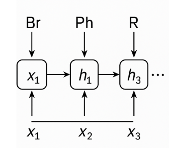
Figure 1: The reaction is encoded as a sequence of tokens. At each step t, the input token 𝑥_𝑡 (e.g., “Br”, “Ph”, “R”) enters an RNN cell. That cell combines the new input with the previous hidden state hₜ₋₁ to produce the updated hidden state hₜ. Arrows show the flow: horizontal arrows carry the hidden state forward through time, and vertical arrows inject each new chemistry token into the cell. This illustrates how the network incrementally builds a memory of the reaction’s components, accumulating context that will ultimately be used to predict the reaction’s yield.

In summary, an RNN reads a reaction like a chemist reads a procedure, forming an expectation of yield as it goes. This approach can capture nuanced patterns (like synergistic effects of reagents) that might be hard to encode with fixed descriptors.

Why RNNs Succeed (and Where They Struggle)

Advantage

RNNs excel at capturing sequential patterns. In chemistry, this means they naturally take into account the presence and context of each component in a reaction. They can, for example, learn that “having ligand X together with base Y” is a pattern associated with high yield, whereas models that treat X and Y as independent features might miss that interaction.

Limitations

• Data Requirements: RNNs are data-hungry and require many examples to train well. If we had a much smaller dataset, an RNN might overfit or fail to learn meaningful patterns.
• Vanishing Gradients on Long Sequences: Standard RNNs can struggle with very long sequences due to vanishing or exploding gradients, making it hard to learn long-range dependencies. Architectural improvements like LSTM mitigate this but add complexity.
• Complexity for Beginners: The mathematical formulation of RNNs (with looping states and backpropagation through time) is more complex than a simple feed-forward network. This can be challenge for those new to machine learning.

Implementation Example: RNN for Yield Prediction

Let’s walk through an example of building and training an RNN model to predict reaction yields using Python and PyTorch. We will use a real-world dataset for demonstration. For instance, the Buchwald– Hartwig amination HTE dataset (Ahneman et al., Science 2018) contains thousands of C–N cross-coupling reactions with measured yields. Each data point in this dataset is a reaction (specific aryl halide, amine, base, ligand, etc.) and the resulting yield.

1. Set Up The Environment

• Open google-colab/Python
• Instal core packages for RNN:

    pip install torch torchvision torchaudio  
    pip install pandas scikit-learn matplotlib requests   
  

• Install chemistry helpers package:

    pip intall rdkit
  

2. Download the dataset

Download Buchwald-Hartwig dataset then store in “yield_data.csv” file

    import requests
    url = "https://raw.githubusercontent.com/rxn4chemistry/rxn_yields/master/data/Buchwald-Hartwig/Dreher_and_Doyle_input_data.xlsx"
    resp = requests.get(url)
    with open("yield_data.csv", "wb") as f:
        f.write(resp.content)
    print("Dataset downloaded and saved as yield_data.csv")

3. Get helpers function and generate reaction SMILES

Transforms the spreadsheet style HTE dataset into standard reaction SMILES format

from rdkit import Chem
from rdkit.Chem import rdChemReactions

def canonicalize_with_dict(smi, can_smi_dict={}):
    if smi not in can_smi_dict.keys():
        return Chem.MolToSmiles(Chem.MolFromSmiles(smi))
    else:
        return can_smi_dict[smi]

def generate_buchwald_hartwig_rxns(df):
    """
    Converts the entries in the excel files from Sandfort et al. to reaction SMILES.
    """
    df = df.copy()
    fwd_template = '[F,Cl,Br,I]-[c;H0;D3;+0:1](:[c,n:2]):[c,n:3].[NH2;D1;+0:4]-[c:5]>>[c,n:2]:[c;H0;D3;+0:1](:[c,n:3])-[NH;D2;+0:4]-[c:5]'
    methylaniline = 'Cc1ccc(N)cc1'
    pd_catalyst = Chem.MolToSmiles(Chem.MolFromSmiles('O=S(=O)(O[Pd]1~[NH2]C2C=CC=CC=2C2C=CC=CC1=2)C(F)(F)F'))
    methylaniline_mol = Chem.MolFromSmiles(methylaniline)
    rxn = rdChemReactions.ReactionFromSmarts(fwd_template)
    products = []
    for i, row in df.iterrows():
        reacts = (Chem.MolFromSmiles(row['Aryl halide']), methylaniline_mol)
        rxn_products = rxn.RunReactants(reacts)

        rxn_products_smiles = set([Chem.MolToSmiles(mol[0]) for mol in rxn_products])
        assert len(rxn_products_smiles) == 1
        products.append(list(rxn_products_smiles)[0])
    df['product'] = products
    rxns = []
    can_smiles_dict = {}
    for i, row in df.iterrows():
        aryl_halide = canonicalize_with_dict(row['Aryl halide'], can_smiles_dict)
        can_smiles_dict[row['Aryl halide']] = aryl_halide
        ligand = canonicalize_with_dict(row['Ligand'], can_smiles_dict)
        can_smiles_dict[row['Ligand']] = ligand
        base = canonicalize_with_dict(row['Base'], can_smiles_dict)
        can_smiles_dict[row['Base']] = base
        additive = canonicalize_with_dict(row['Additive'], can_smiles_dict)
        can_smiles_dict[row['Additive']] = additive

        reactants = f"{aryl_halide}.{methylaniline}.{pd_catalyst}.{ligand}.{base}.{additive}"
        rxns.append(f"{reactants}>>{row['product']}")
    return rxns

4. Preprocessing & Data Preparation

We will load the raw Excel file, generate reaction SMILES, split into train/test, build a character‑level vocabulary, and wrap everything in PyTorch format so that we could run on RNN model later.

import pandas as pd
import torch
from sklearn.model_selection import train_test_split
from torch.utils.data import Dataset, DataLoader
from torch.nn.utils.rnn import pad_sequence

# 1.1  Read the Excel file from `yield_data.xlsx`
df = pd.read_excel('yield_data.csv', sheet_name='FullCV_01')

# 1.2 Convert each row’s reagent columns into a single reaction SMILES string
df['rxn_smiles'] = generate_buchwald_hartwig_rxns(df)

# 1.3 Keep only the SMILES and the yield column (rename to 'yield')
data = df[['rxn_smiles', 'Output']].rename(columns={'Output': 'yield'})

# 1.4 Split into train/test
train_df, test_df = train_test_split(data, test_size=0.2, random_state=42)

# 1.5 Build a char‑level vocabulary (PAD token at index 0)
chars = sorted({ch for smi in train_df.rxn_smiles for ch in smi})
chars = ['<PAD>'] + chars
vocab  = {ch: i for i, ch in enumerate(chars)}
PAD_IDX = 0

def encode(smi):
    return [vocab[ch] for ch in smi]

# 1.6 Define a Dataset that pads & scales yields 0–1
class RxnDataset(Dataset):
    def __init__(self, df):
        self.seqs   = [torch.tensor(encode(s), dtype=torch.long) for s in df.rxn_smiles]
        self.length = [len(s) for s in self.seqs]
        self.y      = torch.tensor(df['yield'].values / 100, dtype=torch.float32)
    def __len__(self):
        return len(self.seqs)
    def __getitem__(self,idx):
        return self.seqs[idx], self.length[idx], self.y[idx]


def collate(batch):
    seqs, lens, ys = zip(*batch)
    seq_pad = pad_sequence(seqs, batch_first=True, padding_value=PAD_IDX)
    lens    = torch.tensor(lens)
    ys      = torch.tensor(ys)
    return seq_pad, lens, ys

train_loader = DataLoader(RxnDataset(train_df), batch_size=32, shuffle=True, collate_fn=collate)
test_loader  = DataLoader(RxnDataset(test_df),  batch_size=32, shuffle=False, collate_fn=collate)

5. Create RNN model

We define an LSTM‑based RNN that:

• Embeds each token ID → vector

• Runs a packed LSTM over the sequence (skipping PADs)

• Reads out the final hidden state → linear layer → predicted yield (0–1)

import torch.nn as nn
from torch.nn.utils.rnn import pack_padded_sequence

class YieldRNN(nn.Module):
    def __init__(self, vocab_size, embed_dim=64, hidden_dim=256):
        super().__init__()
        self.embed = nn.Embedding(vocab_size, embed_dim,
                                  padding_idx=PAD_IDX)
        self.lstm  = nn.LSTM(embed_dim, hidden_dim,
                             batch_first=True)
        self.fc    = nn.Linear(hidden_dim, 1)

    def forward(self, x, lengths):
        # x: (batch, seq_len); lengths: (batch,)
        emb = self.embed(x) 
        packed = pack_padded_sequence(
            emb, lengths.cpu(),
            batch_first=True,
            enforce_sorted=False
        )
        _, (h, _) = self.lstm(packed)
        # h[-1]: final hidden state of last LSTM layer → (batch, hidden_dim)
        return self.fc(h[-1]).squeeze(1)

6. Training & Evaluation

Here we train for 300 epochs with MSE loss (on scaled 0–1 yields), print train and validation MSE every 10 epochs.

import torch
import matplotlib.pyplot as plt
import numpy as np
import math

# Using GPU instead of CPU if possible
device = 'cuda' if torch.cuda.is_available() else 'cpu'
model = YieldRNN(len(vocab)).to(device)
criterion = nn.MSELoss()
optim     = torch.optim.Adam(model.parameters(), lr=1e-3)

# Training loop
for epoch in range(300):
    model.train()
    train_mse, n_train = 0.0, 0
    for X, L, y in train_loader:
        X, L, y = X.to(device), L.to(device), y.to(device)
        optim.zero_grad()
        pred = model(X, L)
        loss = criterion(pred, y)
        loss.backward()
        optim.step()
        train_mse += loss.item() * y.size(0)
        n_train   += y.size(0)
    train_mse /= n_train
    # ---- validation every 10 epochs ----
    if epoch % 10 == 0:
        model.eval(); mse = 0; n = 0
        with torch.no_grad():
            for X, L, y in test_loader:
                X, L, y = X.to(device), L.to(device), y.to(device)
                mse += criterion(model(X, L), y).item() * len(y)
                n  += len(y)
        print(f"Epoch {epoch:3d} Train MSE: {train_mse}  Val MSE: {mse/n:.4f} ")

6. Model Evaluation on the Test Set

Once training is complete, we switch the model into evaluation mode and measure how well it predicts unseen reactions:

model.eval()
preds, trues = [], []
with torch.no_grad():
    for X, L, y in test_loader:
        X, L = X.to(device), L.to(device)
        preds.extend(model(X, L).cpu().numpy() * 100)
        trues.extend(y.numpy() * 100)

import numpy as np, matplotlib.pyplot as plt, math
preds, trues = np.array(preds), np.array(trues)
rmse = math.sqrt(((preds - trues)**2).mean())
print(f"RMSE on test set: {rmse:.1f}% yield")

plt.scatter(trues, preds, alpha=0.6, edgecolors='k')
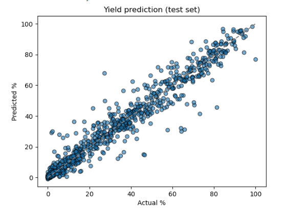
plt.plot([0,100],[0,100],'--',c='gray'); plt.xlabel('Actual %'); plt.ylabel('Predicted %')
plt.title('Yield prediction (test set)')
plt.show()

from sklearn.metrics import r2_score

r2 = r2_score(np.array(trues), np.array(preds))
print(f"R² on test set: {r2:.3f}")

Output: After training for 300 epochs, the model converged to a stable performance on the held‑out test set:

• Validation convergence:
  • Final validation MSE ≈ 0.0030
  • Corresponding RMSE ≈ √0.0030 ≈ 0.055 → 5.5 % yield error
• Test‐set metrics
  • RMSE on test set: 5.2% yield
  • R² on test set: 0.957
• Interpretation
  • An RMSE of 5.2 % means that, on average, the model’s predicted yields deviate from the true yields by just over ±5 percentage points. The level of accuracy on par with many published HTE yield‐prediction models.
  • An R² of 0.957 indicates the network captures 95.7 % of the variance in experimental yields, demonstrating strong predictive power.
• Scatter plot
  

Section 8.1 – Quiz Questions

1) Factual Questions

Question 1

Which PyTorch class provides a fully connected layer that applies a linear transformation to input data?
A. nn.Linear
B. nn.RNN
C. nn.Conv1d
D. nn.BatchNorm1d

Question 2

A common training problem with vanilla RNNs on very long sequences is:
A. Over-smoothing of graph topology
B. Vanishing or exploding gradients
C. Excessive GPU memory during inference
D. Mandatory one-hot encoding of inputs

2) Comprehension / Application Questions

Question 3

Which of the following is an example application of RNNs?
A. Modeling atom-level interactions in molecular graphs
B. Modeling reaction kinetics in continuous pharmaceutical manufacturing
C. Classifying reaction product color from images
D. Embedding molecules using graph convolutional layers

Question 4

If you change hidden_dim from 64 → 32 without altering anything else, you primarily reduce:
A. The number of time-steps processed
B. Model capacity (fewer parameters)
C. Training epochs required
D. Sequence length

8.2 Graph Neural Networks (GNNs)

Why Use GNNs for Yield Prediction?

While RNNs treat reactions as sequences of characters, Graph Neural Networks (GNNs) treat chemical structures as graphs of atoms and bonds. In a molecular graph, nodes represent atoms and edges represent bonds. GNNs are a natural choice for chemistry because they can directly use the connectivity information of molecules. For yield prediction, GNNs can encode detailed structural features that influence reactivity. For example, things like steric hindrance (crowdedness around a reactive site), electronic effects transmitted through a conjugated system, or the presence of particular substructures, all by the way the graph is connected.

Importantly, GNNs produce learned molecular descriptors. Instead of us defining features (like molecular weight), a GNN can learn its own features by message passing on the graph. This is advantageous when predicting yields because subtle structural features or combinations of features that affect yield can be discovered by the model. For example, a GNN might learn a specific combination of a leaving group and a neighboring substituent that tends to reduce yield, something that would be hard to capture in a single traditional descriptor.

Another strength is that GNNs naturally handle variable-sized structures. Whether a molecule has 10 atoms or 50, a graph network can process it (by iterating over the actual bonds), and produce a fixed-size vector representation for it. This is ideal for reaction data where different entries may have very different substrates. GNNs also uphold the principle that isomorphic graphs (chemically identical molecules) produce the same representation, regardless of how atoms are indexed in the input . This is important for chemistry, where the numbering of atoms in a file is irrelevant, only the bonding matters.

In summary, GNNs bring chemical perception to yield prediction: they view molecules the way a chemist does, as collections of atoms connected in a particular way, and can therefore learn reactivity trends that arise from molecular structure.

How GNNs Work

A GNN operates by letting atoms in a molecule talk to their neighbors through a series of messagepassing steps. Initially, each atom is described by some feature vector (for example, one could start with a one-hot encoding of the atom’s element type, or include other basic info like how many hydrogens it has). In the first message passing round, each atom sends a message to its directly bonded neighbors – this message could be a trainable function of the atom’s current state and perhaps the bond type. The neighbors receive these messages and update their own state (often by summing or averaging the incoming messages). This is one graph convolution or message-passing layer. Then the process repeats for multiple layers. With each layer, information spreads outward: after layers, each atom’s state contains information about atoms up to bonds away.

For a reaction yield prediction, we might construct a graph that includes all reactant and reagent molecules in one big disconnected graph (each separate molecule is a component of the graph). Messages will propagate within each molecule, and potentially we could also allow some global node or cross-coupling if modeling interactions between molecules (some advanced approaches add “reaction condition nodes” or connect all components to a dummy node to allow inter-molecular effects). Most simply, we treat each molecule separately and then combine their learned representations.

After message passing, we need a fixed-size representation for the whole reaction. Commonly, GNNs use a readout or pooling step: for example, take the final state of all atoms in a molecule and either average them or take the sum. This produces a vector representation for each molecule. If multiple molecules are present (multiple reactants), those vectors might be concatenated or summed to represent the entire reaction. Finally, this reaction-level vector is fed into a predictive model (like a feed-forward layer) to output the yield.

Key intuition: GNNs can learn chemistry rules. For instance, it might learn a node update rule that when a nitrogen (in a base) is adjacent to a bulky substituent, the message it sends indicates “I’m a hindered base” which might be correlated with lower yield. Or an aryl halide node might send a message to its neighbors indicating “I’m an electron-poor (or electron-rich) ring”, affecting how the palladium catalyst would oxdiatively insert, and thus yield. After training on many examples, these learned messages and node states encode what substructures and connectivity patterns are favorable or unfavorable for the reaction.

Implementing a GNN for Yield Prediction

Let’s outline how we could train a GNN on the same Buchwald-Hartwig dataset. Instead of feeding sequences to a model, we will feed molecular graphs. One approach is to use a library like Deep Graph Library (DGL) or PyTorch Geometric for convenience.

Below is a full PyTorch Geometric workflow with the same “lab notebook” style used in the RNN section. Each step can be pasted into a Colab or local notebook to download the Buchwald–Hartwig dataset, convert molecules into graphs, and train a 3-layer GCN to regress the yields.

0. Install dependencies (Colab / fresh env)

!pip install torch torchvision torchaudio
!pip install rdkit-pypi
!pip install torch_geometric torch-scatter torch-sparse torch-cluster torch-spline-conv -q

1. Imports environments

import os
import math
import requests
import numpy as np
import pandas as pd
from rdkit import Chem

import torch
import torch.nn as nn
import torch.nn.functional as F

from torch_geometric.data import Data
from torch_geometric.loader import DataLoader
from torch_geometric.nn import GCNConv, global_mean_pool
from sklearn.metrics import r2_score
# Choose the device to train the model
if torch.cuda.is_available():
    device = torch.device("cuda")
else:
    device = torch.device("cpu")
print("Using device:", device)

2. Download the dataset

url = "https://raw.githubusercontent.com/rxn4chemistry/rxn_yields/master/data/Buchwald-Hartwig/Dreher_and_Doyle_input_data.xlsx"
fname = "buchwald_hartwig_data.xlsx"

if not os.path.exists(fname):
    resp = requests.get(url)
    with open(fname, "wb") as f:
        f.write(resp.content)
    print("Downloaded dataset.")
else:
    print("Dataset already exists.")

df = pd.read_excel(fname, sheet_name="FullCV_01")
print("Loaded", len(df), "rows")
print(df.head())

3. Convert molecules to PyG graphs

# Atom types to one-hot encode (others go to "other" bucket)
ALLOWED_ATOMS = [1, 6, 7, 8, 9, 15, 16, 17, 35, 53]  # H, C, N, O, F, P, S, Cl, Br, I

def atom_features(atom):
    """Simple one-hot on element type + aromatic flag."""
    Z = atom.GetAtomicNum()
    atom_type = [int(Z == z) for z in ALLOWED_ATOMS]
    if sum(atom_type) == 0:
        atom_type.append(1)
    else:
        atom_type.append(0)
    aromatic = [int(atom.GetIsAromatic())]
    return torch.tensor(atom_type + aromatic, dtype=torch.float)

def mol_to_graph(mol, offset=0):
    """RDKit mol -> (node_features, edge_index). offset shifts atom indices."""
    if mol is None:
        return None, None
    num_atoms = mol.GetNumAtoms()
    if num_atoms == 0:
        return None, None

    x_list = [atom_features(mol.GetAtomWithIdx(i)) for i in range(num_atoms)]
    x = torch.stack(x_list, dim=0) 

    # bonds -> undirected edges
    edge_index = []
    for bond in mol.GetBonds():
        i = bond.GetBeginAtomIdx() + offset
        j = bond.GetEndAtomIdx() + offset
        edge_index.append([i, j])
        edge_index.append([j, i])
    if len(edge_index) == 0:
        # isolated atom/fragment; still create something
        edge_index = torch.empty((2, 0), dtype=torch.long)
    else:
        edge_index = torch.tensor(edge_index, dtype=torch.long).t().contiguous()
    return x, edge_index


def reaction_row_to_graph(row):
    """
    Build a reaction-level graph from the four varying components.
    We create one big graph that is just the disjoint union of:
        Aryl halide + Ligand + Base + Additive
    """
    smiles_list = [
        row.get("Aryl halide", ""),
        row.get("Ligand", ""),
        row.get("Base", ""),
        row.get("Additive", ""),
    ]

    all_x = []
    all_edges = []
    offset = 0

    for smi in smiles_list:
        if not isinstance(smi, str) or smi.strip() == "":
            continue
        mol = Chem.MolFromSmiles(smi)
        x, e = mol_to_graph(mol, offset=offset)
        if x is None:
            continue
        all_x.append(x)
        if e.numel() > 0:
            all_edges.append(e)
        offset += x.size(0)

    if len(all_x) == 0:
        return None  

    x_all = torch.cat(all_x, dim=0)
    if len(all_edges) == 0:
        edge_index = torch.empty((2, 0), dtype=torch.long)
    else:
        edge_index = torch.cat(all_edges, dim=1)

    y = torch.tensor([row["Output"] / 100.0], dtype=torch.float32)
    data = Data(x=x_all, edge_index=edge_index, y=y)
    return data

4. Build the full PyG dataset and split 80/20

data_list = []
for idx, row in df.iterrows():
    g = reaction_row_to_graph(row)
    if g is not None:
        data_list.append(g)

print(f"Built graphs for {len(data_list)} reactions (out of {len(df)})")

from sklearn.model_selection import train_test_split

num_graphs = len(data_list)
indices = np.arange(num_graphs)
train_idx, test_idx = train_test_split(indices, test_size=0.2, random_state=42, shuffle=True)

train_list = [data_list[i] for i in train_idx]
test_list  = [data_list[i] for i in test_idx]

train_loader = DataLoader(train_list, batch_size=64, shuffle=True)
test_loader  = DataLoader(test_list,  batch_size=64, shuffle=False)

num_node_features = train_list[0].x.size(1)
print("Node feature dimension:", num_node_features)

5. Define the graph neural network

We will implement a small GNN with two graph convolution layers. Each layer will update atom features by incorporating information from neighbor atoms (using, a GraphConv which is a common graph convolution operation).

class YieldGNN(nn.Module):
    def __init__(self, in_channels, hidden_channels=64):
        super().__init__()
        self.conv1 = GCNConv(in_channels, hidden_channels)
        self.conv2 = GCNConv(hidden_channels, hidden_channels)
        self.conv3 = GCNConv(hidden_channels, hidden_channels)

        self.lin1 = nn.Linear(hidden_channels, 64)
        self.lin2 = nn.Linear(64, 1)

    def forward(self, x, edge_index, batch):
        x = self.conv1(x, edge_index)
        x = F.relu(x)
        x = self.conv2(x, edge_index)
        x = F.relu(x)
        x = self.conv3(x, edge_index)
        x = F.relu(x)

        x = global_mean_pool(x, batch)  

        x = F.relu(self.lin1(x))
        out = self.lin2(x)             
        return out.view(-1)     


model = YieldGNN(num_node_features).to(device)
criterion = nn.MSELoss()
optimizer = torch.optim.Adam(model.parameters(), lr=1e-3)

print(model)

6. Train and evaluate

We would train this GNN similar to how we trained the RNN: use an MSE loss between predicted and true yields, and an optimizer like Adam. The training loop would iterate over each reaction graph. DGL can provide a GraphDataLoader to batch multiple small graphs together for efficiency.

def train_one_epoch():
    model.train()
    total_loss = 0.0
    n = 0
    for batch in train_loader:
        batch = batch.to(device)
        optimizer.zero_grad()
        pred = model(batch.x, batch.edge_index, batch.batch)
        y = batch.y.view(-1).to(device)
        loss = criterion(pred, y)
        loss.backward()
        optimizer.step()
        total_loss += loss.item() * y.size(0)
        n += y.size(0)
    return total_loss / n

def evaluate(loader):
    model.eval()
    preds = []
    trues = []
    with torch.no_grad():
        for batch in loader:
            batch = batch.to(device)
            pred = model(batch.x, batch.edge_index, batch.batch)
            y = batch.y.view(-1)
            preds.append(pred.cpu())
            trues.append(y.cpu())
    preds = torch.cat(preds).numpy() * 100.0
    trues = torch.cat(trues).numpy() * 100.0
    rmse = math.sqrt(np.mean((preds - trues) ** 2))
    r2 = r2_score(trues, preds)
    return rmse, r2

num_epochs = 60
for epoch in range(1, num_epochs + 1):
    train_mse = train_one_epoch()
    if epoch % 10 == 0 or epoch == 1:
        rmse, r2 = evaluate(test_loader)
        print(f"Epoch {epoch:3d} | Train MSE (scaled): {train_mse:.4f} | "
              f"Test RMSE: {rmse:.2f}% | R²: {r2:.3f}")

rmse, r2 = evaluate(test_loader)
print(f"\nFinal Test RMSE: {rmse:.2f}% yield")
print(f"Final Test R²: {r2:.3f}")

Expected performance: Graph-based models have also been shown to achieve strong performance on this dataset. We would expect a well-tuned GNN to also reach an RMSE in the mid single-digits (% yield). For example, a message-passing neural network in one study achieved around 5–6% RMSE, comparable to the RNN and Random Forest models. The advantage of the GNN might emerge more in scenarios where we want to generalize to novel structures or when the dataset features a lot of structural diversity, the GNN’s learned representation can be more directly tied to chemical features (like functional groups) than an RNN’s sequence-based representation.

Advantages and Limitations of GNNs

Advantages:

GNNs leverage rich structural information. They do not require us to decide which chemical features are important. Instead, they can learn complex combinations of atomic features and connectivity that correlate with yield. They are invariant to atom indexing and molecular size, making them very flexible. For multi-component reactions, GNNs can even capture interactions between different molecules. Notably, GNNs have been successful in many chemical property predictions, and yield prediction is no exception. They can outperform fixed-descriptor models especially when there are enough data to learn subtle structure-property relationships.

Limitations:

GNN models can be more complex and sometimes harder to interpret. While an RNN might tell us “this substring pattern was important” a GNN’s learned weights are spread across many message functions. We might need additional tools (like attention mechanisms) to extract chemical insights. GNNs also often require more computational effort per example than simpler models, especially for large molecules or many message passing steps. Another limitation is that GNNs typically consider 2D graph structure. They may ignore 3D conformational effects unless explicitly included (there are 3D message passing networks, but those need 3D coordinates which are not always available). In the context of yield, if stereochemistry or conformation plays a big role, a plain 2D GNN might miss it unless those factors are encoded somehow.

In summary, GNNs provide a way for the model to “learn chemistry” from the data, figuring out which atomic connections enhance or suppress yields. They are a powerful tool especially as reaction datasets grow and encompass diverse chemistry where knowing the connectivity is key.

Section 8.2 – Quiz Questions (Graph Neural Networks)

1) Factual Questions

Question 1

In a molecular graph, nodes typically represent:
A. Bonds
B. Atoms
C. Ring systems
D. IR peaks

Question 2

A key advantage of GNNs for chemistry is their ability to:
A. Ignore local atomic environments
B. Map variable-size molecules to fixed-length vectors
C. Require explicit reaction conditions
D. Operate only on tabular data

2) Comprehension / Application Questions

Question 3

You have reaction data but only in the form of reactant SMILES (no 3D coordinates). Can you still train a GNN to predict yields? A. Yes, 2D graph connectivity (from SMILES) is usually enough to start with B. No, GNNs strictly require 3D geometry C. Only after performing quantum calculations for each reactant D. Only if you convert each SMILES to an image first

Question 3

Which factor is not an inherent limitation or consideration of graph neural networks in chemistry?
A. Difficulty in interpreting what the model has learned B. Inability to handle molecules with many atoms C. Potential to miss effects of molecular conformations (3D) if only 2D is used D. Higher computational cost per molecule compared to simple fingerprint models

8.3 Random Forests

Why Use Random Forests for Yield Prediction?

Random Forests are a popular ensemble learning method that often serve as a strong baseline for many prediction tasks, including reaction yields . A random forest is essentially a collection of decision trees (hence “forest”) where each tree votes on the prediction. They work with fixed-size feature vectors rather than sequences or graphs. In the context of yield prediction, this means we first need to represent each reaction with a set of numerical descriptors or features.

Historically, many chemistry researchers have hand-crafted or computed descriptors for reactions: for example, electronic and steric parameters of substituents, solvent polarity indices. In the Buchwald-Hartwig example, Ahneman et al. computed dozens of features for each reaction component(like atomic charges, bond distances from DFT calculations) and concatenated them into one large feature vector. They then trained a random forest on these vectors to predict yield, and found it outperformed linear regression significantly.

The appeal of random forests in chemistry is that they are relatively robust and require minimal hyperparameter tuning. They can handle nonlinear relationships and interactions between features, but they won’t overfit badly if you grow enough trees with proper settings. For yield prediction, if you have a moderate-sized dataset (say a few hundred or a few thousand reactions) and a good set of features, a random forest often does a very good job. It can capture patterns like “if feature X (e.g., electronegativity of a substituent) is above some threshold and feature Y (e.g., catalyst type) is a certain category, then yields tend to be high”, essentially the decision trees partition the feature space into regions corresponding to different yield outcomes.

Another big advantage: interpretability. Random forests can give you measures like feature importance, indicating which descriptors most strongly influence the yield prediction. This can sometimes align with chemical intuition (e.g., it might highlight that “ligand bite angle” or “substrate steric bulk” were important features).

However, a limitation is that you only learn from what you explicitly describe in the features. If a crucial aspect of the chemistry is not encoded (for example, you did not include a descriptor capturing some subtle interaction), the model can’t learn it. This is where the deep learning models (RNNs, GNNs) have an edge by learning representations automatically. But for many cases, carefully chosen descriptors + random forest remain a very effective solution, especially when data is limited.

How Random Forests Work

A single decision tree splits the data based on feature values. For example, it might first split on “Ligand = bulky vs not bulky”, then within the “bulky” branch split on “Base pKa > X or <= X”, and so on, eventually reaching a small group of training points at each leaf which is used to make a prediction (like the average yield of that group). Decision trees tend to overfit if grown deep, but a random forest combats this by averaging many trees . Each tree in the forest is trained on a slightly different subset of the data and typically a different subset of features for each split. This “randomness” ensures the trees are diverse. When we predict, each tree gives a vote and the forest outputs the average of all trees’ outputs.

The result is a stable predictor that usually has better generalization than a single tree, and it can model complex nonlinear relationships without a lot of parameter fiddling.

Implementing a Random Forest for Yield

Random Forests are a strong non-neural baseline for yield prediction: they work well on small/medium tabular datasets, require little tuning, and give chemists a fast way to see whether simple descriptors already capture most of the yield signal.

Below is an example of training a Random Forest regressor on the Buchwald–Hartwig HTE dataset.

0. Install dependencies (once per environment)

!pip install pandas scikit-learn rdkit-pypi requests matplotlib

1. Imports libraries

import os
import math
import requests
import numpy as np
import pandas as pd

from rdkit import Chem
from rdkit.Chem import AllChem
from rdkit import DataStructs

from sklearn.ensemble import RandomForestRegressor
from sklearn.model_selection import train_test_split
from sklearn.metrics import r2_score, mean_squared_error

2. Download Buchwald–Hartwig dataset

url = "https://raw.githubusercontent.com/rxn4chemistry/rxn_yields/master/data/Buchwald-Hartwig/Dreher_and_Doyle_input_data.xlsx"
fname = "buchwald_hartwig_data.xlsx"

if not os.path.exists(fname):
    resp = requests.get(url)
    with open(fname, "wb") as f:
        f.write(resp.content)
    print("Downloaded dataset.")
else:
    print("Dataset already exists.")

# Load one fold
df = pd.read_excel(fname, sheet_name="FullCV_01")

3. Build reaction-level Morgan fingerprints

def reaction_to_morgan_fp(row, radius=2, n_bits=2048):
    """
    Combine all varying reactants/reagents into one "mixture" molecule
    then compute a single Morgan fingerprint.
    """
    smiles_list = [
        row.get("Aryl halide", ""),
        row.get("Ligand", ""),
        row.get("Base", ""),
        row.get("Additive", ""),
    ]

    mols = []
    for smi in smiles_list:
        if not isinstance(smi, str) or smi.strip() == "":
            continue
        mol = Chem.MolFromSmiles(smi)
        if mol is not None:
            mols.append(mol)

    if not mols:
        return None

    combo = mols[0]
    for mol in mols[1:]:
        combo = Chem.CombineMols(combo, mol)

    fp = AllChem.GetMorganFingerprintAsBitVect(combo, radius, nBits=n_bits)
    arr = np.zeros((n_bits,), dtype=int)
    DataStructs.ConvertToNumpyArray(fp, arr)
    return arr


X_list, y_list = [], []
for _, row in df.iterrows():
    fp = reaction_to_morgan_fp(row)
    if fp is None:
        continue
    X_list.append(fp)
    y_list.append(row["Output"])

X = np.vstack(X_list)
y = np.array(y_list)

print("Feature matrix shape:", X.shape)
print("Targets shape:", y.shape)

4.Train test split

X_train, X_test, y_train, y_test = train_test_split(
    X, y, test_size=0.2, random_state=42
)

5. Train Random Forest regressor

rf = RandomForestRegressor(
    n_estimators=100,
    max_depth=None,
    min_samples_leaf=1,
    n_jobs=-1,
    oob_score=True,
    random_state=0,
)
rf.fit(X_train, y_train)
print(f"OOB R² estimate: {rf.oob_score_:.3f}")

6. Evaluate on the held-out 20 %

y_pred = rf.predict(X_test)
rmse = math.sqrt(mean_squared_error(y_test, y_pred))
r2 = r2_score(y_test, y_pred)

print(f"Random Forest – Test RMSE: {rmse:.2f}% yield")
print(f"Random Forest – Test R²:   {r2:.3f}")

import matplotlib.pyplot as plt
plt.scatter(y_test, y_pred, alpha=0.5, edgecolors="k")
plt.plot([0, 100], [0, 100], "--", color="gray")
plt.xlabel("Actual yield (%)")
plt.ylabel("Predicted yield (%)")
plt.title(f\"Random Forest – Buchwald–Hartwig\\nRMSE={rmse:.1f}%, R²={r2:.3f}\")
plt.show()

One thing to note: the random forest can’t extrapolate beyond the chemistry it has seen. If a certain functionalgroup never appears in the training data, the model has no basis to predict its effect on yield (other than whatever default bias it has learned). In contrast, a GNN or RNN that embeds substructures mightgeneralize a bit better by understanding similarities. That said, within the domain of the training data,random forests often do as well as more complex models and are much faster to train.

Advantages and Limitations of Random Forests

Advantages:

• Ease of use: They work out-of-the-box with minimal tuning. No need for extensive architecture design.
• Interpretability: Decision trees and ensembles of them can provide insight. You can calculate feature importance or even inspect individual trees to see what splits they learned (though a forest with 100 trees is cumbersome to fully interpret).
• Small data friendly: They don’t require massive datasets, even with a few hundred data points, a random forest can perform decently, whereas deep models might overfit.
• Fast prediction: After training, making predictions with a random forest is usually very fast, which is useful for screening large reaction spaces.

Limitations:

• Feature engineering required: You must decide how to represent the reaction. The model itself won’t invent new features. It only knows what you feed it. If the fingerprint or descriptors miss a key aspect (e.g., whether the reaction is intramolecular or not), the forest can’t compensate.
• Curse of dimensionality: If you use very high-dimensional fingerprints with lots of bits, many of them might be irrelevant. Random forests handle this better than linear models (they’ll just tend to ignore useless features), but extremely sparse, high-d dimensions can still be problematic unless you have lots of data.
• Not sequence or graph native: Unlike RNNs or GNNs, forests can’t directly use structured data. We had to flatten the chemistry into a vector. This means some relational information could be lost or diluted. For example, the descriptors might not explicitly encode which ligand was paired with which base in a particular instance, whereas a structured model might. Moreover, the random forest can’t extrapolate beyond the chemistry it has seen.

In practice, random forests became a go-to method in many early machine learning for chemistry papers because of their solid performance and simplicity. Even today, they’re a great baseline, if your fancy new deep model can’t beat the humble random forest, you might reconsider your approach!

Section 8.3 – Quiz Questions (Random Forests)

1) Factual Questions

Question 1

Random Forests are an ensemble of what base learners?
A. Linear regressors
B. Decision trees
C. k-Means clusters
D. Support-vector machines

Question 2

In the scikit-learn RandomForestRegressor, The attribute oob_score_ represents? :
A. Over-optimised benchmark
B. Out-of-bag R² estimate
C. Observed-only bias
D. Objective batching ratio

Question 3

Which hyper-parameter chiefly controls tree diversity in a Random Forest?
A. n_estimators
B. criterion
C. max_depth
D. random_state

2) Comprehension / Application Questions

Question 4

Why are Random Forests a popular choice as a baseline for reaction yield prediction (or other chemistry regressions) when data is limited?
A. They need deep chemical insight
B. They train quickly, handle many feature types, and don’t easily overfit small datasets
C. They always out-perform neural networks
D. They can naturally process raw SMILES strings without encoding

Question 5

Your forest overfits. Which tweak most likely reduces overfitting?
A. Increase max_depth
B. Decrease max_depth
C. Disable bootstrapping
D. Remove feature engineering

8.4 Feed-Forward Neural Networks

Why Use Neural Networks (MLPs) for Yield Prediction?

The term “Neural Network” is very broad, here we specifically mean a feed-forward neural network, also known as a multilayer perceptron (MLP), which is the classic fully-connected network architecture (no recurrence or convolution). These networks take a fixed-size input vector (just like random forests do) and pass it through several layers of linear transformations with nonlinear activation functions.

Before the rise of specialized models (RNNs, GNNs, etc.), chemists did experiment with using simple feedforward NNs on chemical data. In yield prediction, an MLP can be used similarly to a random forest: you first compute a set of descriptors or fingerprints for the reaction, and then feed that numerical feature vector into the network, which will output a predicted yield. The network will learn weights that map those features to the target.

Why consider an MLP when we have RF or more complex nets? One reason is that MLPs can, in theory, approximate any nonlinear function given enough neurons/layers. They might detect complex interactions between features that a single decision tree split could not. For example, an MLP could learn a smooth function that gradually increases yield when “electron-withdrawing ability and steric bulk” have certain combined values, whereas a tree might make a hard split. MLPs can also be trained end-to-end with gradient descent, which means if your features are partially learned or require slight adjustment, the network might adjust initial layers (in practice, one could even input the raw structures as bits and hope the network finds patterns, though this is less effective without huge data).

However, a plain MLP has no built-in chemistry knowledge. It doesn’t know about sequences or graphs. It treats the input vector as just a bunch of numbers. So it relies heavily on the quality of the descriptors given. For this reason, when data is limited, often an MLP does not outperform a well-tuned random forest (which is more robust to noise and can better handle irrelevant features). That said, if we have a lot of data, an MLP can shine by finding subtle nonlinear patterns. Also, with modern frameworks, it is easy to add features like uncertainty estimation or to integrate an MLP as part of a larger model (e.g., combining a graph embedding with an MLP).

How a Feed-Forward Neural Network Works

A feed-forward network has layers of neurons. Each neuron in a layer takes a weighted sum of the outputs from the previous layer and passes it through a nonlinear activation (like ReLU). For example, in a simple 2-layer MLP: input features go into the first hidden layer. Then goes into the second layer (which could be the output). For regression, sometimes no activation on output or maybe a linear activation if predicting real numbers. The network learns the weight matrices and biases by minimizing the loss (e.g., MSE between predicted and actual yields) through backpropagation.

Compared to an RNN or GNN, the MLP is “flat”. It does not inherently understand sequences or graphs, just whatever features you feed it. It also has to have a fixed input size (so we can not directly feed variable-length sequences without first converting them to fixed-length vectors like fingerprints or summed embeddings).

One advantage of MLPs is that they are easier to train than RNNs in some cases (no sequential dependencies, no need to worry about time-step-wise backprop). But they can overfit if they have too many parameters relative to data.

Implementing an MLP for Yield Prediction

Below is a notebook-ready code on how to train an MLP. We recycle the Morgan fingerprint featurization from the Random Forest example, but swap the predictor for a modest three-layer MLP trained with Adam.

0. Install dependencies (once per environment)

!pip install pandas scikit-learn rdkit-pypi requests torch torchvision torchaudio

1. Setup & imports

import os
import math
import requests
import numpy as np
import pandas as pd

from rdkit import Chem
from rdkit.Chem import AllChem
from rdkit import DataStructs

import torch
import torch.nn as nn
import torch.nn.functional as F

from sklearn.model_selection import train_test_split
from sklearn.metrics import r2_score, mean_squared_error

if torch.cuda.is_available():
    device = torch.device("cuda")
else:
    device = torch.device("cpu")
print("Using device:", device)

2. Load Buchwald–Hartwig dataset

url = "https://raw.githubusercontent.com/rxn4chemistry/rxn_yields/master/data/Buchwald-Hartwig/Dreher_and_Doyle_input_data.xlsx"
fname = "buchwald_hartwig_data.xlsx"

if not os.path.exists(fname):
    resp = requests.get(url)
    with open(fname, "wb") as f:
        f.write(resp.content)
    print("Downloaded dataset.")
else:
    print("Dataset already exists.")

df = pd.read_excel(fname, sheet_name="FullCV_01")
print("Loaded", len(df), "rows with columns:", list(df.columns))

3. Reaction → fixed-length vector (Morgan fingerprint)

def reaction_to_morgan_fp(row, radius=2, n_bits=2048):
    """
    Build one "reaction mixture" molecule from all varying components
    and compute a single Morgan fingerprint (ECFP-style bit vector).
    """
    smiles_list = [
        row.get("Aryl halide", ""),
        row.get("Ligand", ""),
        row.get("Base", ""),
        row.get("Additive", ""),
    ]

    mols = []
    for smi in smiles_list:
        if not isinstance(smi, str) or smi.strip() == "":
            continue
        m = Chem.MolFromSmiles(smi)
        if m is not None:
            mols.append(m)

    if not mols:
        return None

    combo = mols[0]
    for m in mols[1:]:
        combo = Chem.CombineMols(combo, m)

    fp = AllChem.GetMorganFingerprintAsBitVect(combo, radius, nBits=n_bits)
    arr = np.zeros((n_bits,), dtype=np.float32)
    DataStructs.ConvertToNumpyArray(fp, arr)
    return arr

X_list, y_list = [], []
for _, row in df.iterrows():
    fp = reaction_to_morgan_fp(row)
    if fp is None:
        continue
    X_list.append(fp)
    y_list.append(row["Output"] / 100.0)  # scale yields 0–1 for stability

X = np.vstack(X_list)
y = np.array(y_list)
print("Feature matrix shape:", X.shape)
print("Target shape:", y.shape)

4. Train/test split

X_train, X_test, y_train, y_test = train_test_split(
    X, y, test_size=0.2, random_state=42
)

X_train_t = torch.tensor(X_train, dtype=torch.float32).to(device)
y_train_t = torch.tensor(y_train, dtype=torch.float32).to(device)
X_test_t  = torch.tensor(X_test,  dtype=torch.float32).to(device)
y_test_t  = torch.tensor(y_test,  dtype=torch.float32).to(device)

print("Train size:", X_train_t.shape[0], "Test size:", X_test_t.shape[0])

5. Define the MLP

class YieldMLP(nn.Module):
    def __init__(self, input_dim, hidden_dim=512, hidden_dim2=256, dropout=0.1):
        super().__init__()
        self.fc1 = nn.Linear(input_dim, hidden_dim)
        self.fc2 = nn.Linear(hidden_dim, hidden_dim2)
        self.fc3 = nn.Linear(hidden_dim2, 1)
        self.dropout = nn.Dropout(dropout)

    def forward(self, x):
        x = F.relu(self.fc1(x))
        x = self.dropout(x)
        x = F.relu(self.fc2(x))
        x = self.dropout(x)
        out = self.fc3(x)
        return out.view(-1)


model = YieldMLP(input_dim=X_train_t.shape[1]).to(device)
criterion = nn.MSELoss()
optimizer = torch.optim.Adam(model.parameters(), lr=1e-3)

print(model)

6. Training loop

batch_size = 64
num_epochs = 60

def batched_iter(X_tensor, Y_tensor, batch_size):
    n = X_tensor.size(0)
    perm = torch.randperm(n)
    for start in range(0, n, batch_size):
        idx = perm[start:start + batch_size]
        yield X_tensor[idx], Y_tensor[idx]

for epoch in range(1, num_epochs + 1):
    model.train()
    running_loss = 0.0
    n_seen = 0

    for xb, yb in batched_iter(X_train_t, y_train_t, batch_size):
        optimizer.zero_grad()
        preds = model(xb)
        loss = criterion(preds, yb)
        loss.backward()
        optimizer.step()
        running_loss += loss.item() * yb.size(0)
        n_seen += yb.size(0)

    train_mse = running_loss / n_seen

    if epoch % 10 == 0 or epoch == 1:
        model.eval()
        with torch.no_grad():
            y_pred = model(X_test_t)
            mse = criterion(y_pred, y_test_t).item()
        rmse = math.sqrt(mse) * 100.0  # convert back to %
        r2 = r2_score(
            (y_test_t.cpu().numpy()) * 100,
            (y_pred.cpu().numpy()) * 100,
        )
        print(f"Epoch {epoch:3d} | Train MSE (0–1): {train_mse:.4f} | "
              f"Test RMSE: {rmse:.2f}% | R²: {r2:.3f}")

7. Final evaluation

model.eval()
with torch.no_grad():
    y_pred = model(X_test_t)
    mse = criterion(y_pred, y_test_t).item()

rmse = math.sqrt(mse) * 100.0
r2 = r2_score(
    (y_test_t.cpu().numpy()) * 100,
    (y_pred.cpu().numpy()) * 100,
)
print(f"\nFinal Test RMSE: {rmse:.2f}% yield")
print(f"Final Test R²:   {r2:.3f}")

Advantages and Limitations of Feed-Forward NNs

Advantages:

• Flexible function approximation: An MLP can learn any mapping given enough data and complexity. It can model interactions between input features in ways linear models can not.
• Fast inference: Once trained, computing a yield from an MLP is just a few matrix multiplies, very fast even for large input vectors.
• Can be combined with learned features: In more advanced workflows, one could integrate an MLP with a graph or sequence model. For example, use a GNN to featurize each reactant and then an MLP to predict yield from those features, training all together.
• Well-understood training: We know how to optimize them with backpropagation, and many frameworks make it easy to experiment with layer sizes.

Limitations:

• Data requirements: Neural networks have many parameters. Without enough data, they are prone to overfitting, essentially memorizing the training set rather than learning general patterns. In yield prediction tasks with limited examples, this can be an issue. Regularization strategies (like dropout or weight decay) can help, but there is no guarantee without adequate data.
• No built-in chemistry: The MLP does not know a thing about chemistry. If you permute the input features randomly, it has no way to know (whereas a GNN would be inherently tied to atomic connections). It’s up to the input encoding to make chemical sense.
• Hyperparameter tuning: The performance can depend on choosing the right number of layers, neurons, learning rate. With limited data, tuning these can be tricky (too large and you overfit, too small and you underfit).

In essence, a feed-forward neural network for yield prediction is like a “smart curve-fitting” approach on descriptor space. It can work very well if you have a good descriptor set and decent amount of data, but it often won’t beat more chemically-informed models when data is scarce. Nonetheless, it’s an important component in the toolbox, especially as part of larger deep learning architectures.

Section 8.4 – Quiz Questions (Feed-forward Neural Networks)

1) Factual Questions

Question 1

Which activation function is explicitly used in the MLP snippet?
A. Sigmoid
B. Tanh
C. ReLU
D. Softmax

Question 2

The MLP architecture shown contains how many hidden layers?
A. 1
B. 2
C. 3
D. 0

Question 3

A key limitation of generic feed-forward NNs in chemistry is:
A. Inability to model non-linear relations
B. It requires a fixed-size numerical feature vector, thus losing some structured information
C. It has no trainable parameters so it can’t improve with data
D. It always needs 3D coordinates to work

2) Comprehension / Application Questions

Question 4

If you increase the number of neurons in every hidden layer of an MLP (say from [128, 64] to [256, 128]) without adding more training data, what is a likely outcome?
A. The network might overfit more easily (higher variance)
B. The network will surely train faster
C. The network will become unable to learn the training data
D. The network’s expressive power decreases

Question 5

What operation does nn.MSELoss() perform behind the scenes?
A. Computes cross-entropy between predicted probabilities and one-hot targets
B. Calculates the average of squared differences between predicted and actual values
C. Computes binary cross-entropy loss for binary classification
D. Calculates negative log-likelihood of predicted distributions