3-A. Machine Learning Models
Machine learning (ML) is a subfield of artificial intelligence (AI) focused on developing algorithms and statistical models that enable computers to learn from and make decisions based on data. Unlike traditional programming, where explicit instructions are given, machine learning systems identify patterns and insights from large datasets, improving their performance over time through experience.
ML encompasses various techniques, including supervised learning, where models are trained on labeled data to predict outcomes; unsupervised learning, which involves discovering hidden patterns or groupings within unlabeled data; and reinforcement learning, where models learn optimal actions through trial and error in dynamic environments. These methods are applied across diverse domains, from natural language processing and computer vision to recommendation systems and autonomous vehicles, revolutionizing how technology interacts with the world.
Completed and Compiled Code (3.1): Click Here
3.1 Decision Tree and Random Forest
3.1.1 Decision Trees
Decision Trees are intuitive and powerful models used in machine learning to make predictions and decisions. Think of it like playing a game of 20 questions, where each question helps you narrow down the possibilities. Decision trees function similarly; they break down a complex decision into a series of simpler questions based on the data.
Each question, referred to as a “decision,” relies on a specific characteristic or feature of the data. For instance, if you’re trying to determine whether a fruit is an apple or an orange, the initial question might be, “Is the fruit’s color red or orange?” Depending on the answer, you might follow up with another question—such as, “Is the fruit’s size small or large?” This questioning process continues until you narrow it down to a final answer (e.g., the fruit is either an apple or an orange).
In a decision tree, these questions are represented as nodes, and the possible answers lead to different branches. The final outcomes are represented at the end of each branch, known as leaf nodes. One of the key advantages of decision trees is their clarity and ease of understanding—much like a flowchart. However, they can also be prone to overfitting, especially when dealing with complex datasets that have many features. Overfitting occurs when a model performs exceptionally well on training data but fails to generalize to new or unseen data.
In summary, decision trees offer an intuitive approach to making predictions and decisions, but caution is required to prevent them from becoming overly complicated and tailored too closely to the training data.
3.1.2 Random Forest
Random Forests address the limitations of decision trees by utilizing an ensemble of multiple trees instead of relying on a single one. Imagine you’re gathering opinions about a game outcome from a group of people; rather than trusting just one person’s guess, you ask everyone and then take the most common answer. This is the essence of how a Random Forest operates.
In a Random Forest, numerous decision trees are constructed, each making its own predictions. However, a key difference is that each tree is built using a different subset of the data and considers different features of the data. This technique, known as bagging (Bootstrap Aggregating), allows each tree to provide a unique perspective, which collectively leads to a more reliable prediction.
When making a final prediction, the Random Forest aggregates the predictions from all the trees. For classification tasks, it employs majority voting to determine the final class label, while for regression tasks, it averages the results.
Random Forests typically outperform individual decision trees because they are less likely to overfit the data. By combining multiple trees, they achieve a balance between model complexity and predictive performance on unseen data.
Real-Life Analogy
Consider Andrew, who wants to decide on a destination for his year-long vacation. He starts by asking his close friends for suggestions. The first friend asks Andrew about his past travel preferences, using his answers to recommend a destination. This is akin to a decision tree approach—one friend following a rule-based decision process.
Next, Andrew consults more friends, each of whom poses different questions to gather recommendations. Finally, Andrew chooses the places suggested most frequently by his friends, mirroring the Random Forest algorithm’s method of aggregating multiple decision trees’ outputs.
3.1.3 Implementing Random Forest on the BBBP Dataset
This guide demonstrates how to implement a Random Forest algorithm in Python using the BBBP (Blood–Brain Barrier Permeability) dataset. The BBBP dataset is used in cheminformatics to predict whether a compound can cross the blood-brain barrier based on its chemical structure.
The dataset contains SMILES (Simplified Molecular Input Line Entry System) strings representing chemical compounds, and a target column that indicates whether the compound is permeable to the blood-brain barrier or not.
The goal is to predict whether a given chemical compound will cross the blood-brain barrier, based on its molecular structure. This guide walks you through downloading the dataset, processing it, and training a Random Forest model.
Step 1: Install RDKit (Required for SMILES to Fingerprint Conversion)
We need to use the RDKit library, which is essential for converting SMILES strings into molecular fingerprints, a numerical representation of the molecule.
# Install the RDKit library using pip
!pip install rdkit

from rdkit import Chem
from rdkit.Chem import Draw
# Import the modern fingerprint generator
from rdkit.Chem import rdFingerprintGenerator
import pandas as pd
import numpy as np

# Verify the RDKit installation
print(f"RDKit version: {Chem.rdBase.rdkitVersion}")
Step 2: Download the BBBP Dataset
Instead of a manual download, we can pull the dataset directly from the DeepChem AWS repository. This dataset contains SMILES strings and a target column p_np ($1$ for permeable, $0$ for non-permeable).
# Define the URL for the Blood-Brain Barrier Penetration (BBBP) dataset
url = "https://deepchemdata.s3-us-west-1.amazonaws.com/datasets/BBBP.csv"

# Read the CSV file directly from the URL into a pandas DataFrame
data = pd.read_csv(url)

# Print the first five rows to inspect columns like 'smiles' and 'p_np'
print(data.head())
Step 3: Convert SMILES to Molecular Fingerprints
To use the SMILES strings for modeling, we need to convert them into molecular fingerprints. This process turns the chemical structures into a numerical format that can be fed into machine learning models. We’ll use RDKit to generate these fingerprints using the Morgan Fingerprint method.
# Initialize the generator outside the loop for better efficiency
# radius=2 captures the local neighborhood of each atom
# fpSize=1024 creates a bit-vector of length 1024
mfpgen = rdFingerprintGenerator.GetMorganGenerator(radius=2, fpSize=1024)

def featurize_molecule(smiles):
    """Converts a SMILES string into a Morgan fingerprint bit vector."""
    mol = Chem.MolFromSmiles(smiles)
    if mol:
        # Use the generator object to create the fingerprint
        return mfpgen.GetFingerprint(mol)
    else:
        # Return None if the SMILES string is invalid or cannot be parsed
        return None

# Generate fingerprints for every SMILES string in the dataset
features = [featurize_molecule(smi) for smi in data['smiles']]

# Convert objects to lists, or use a zero-vector for failed molecules
features = [list(fp) if fp is not None else np.zeros(1024) for fp in features]

# Create the final feature matrix X and target vector y
X = np.array(features)
y = data['p_np']
The diagram below provides a visual representation of what this code does:
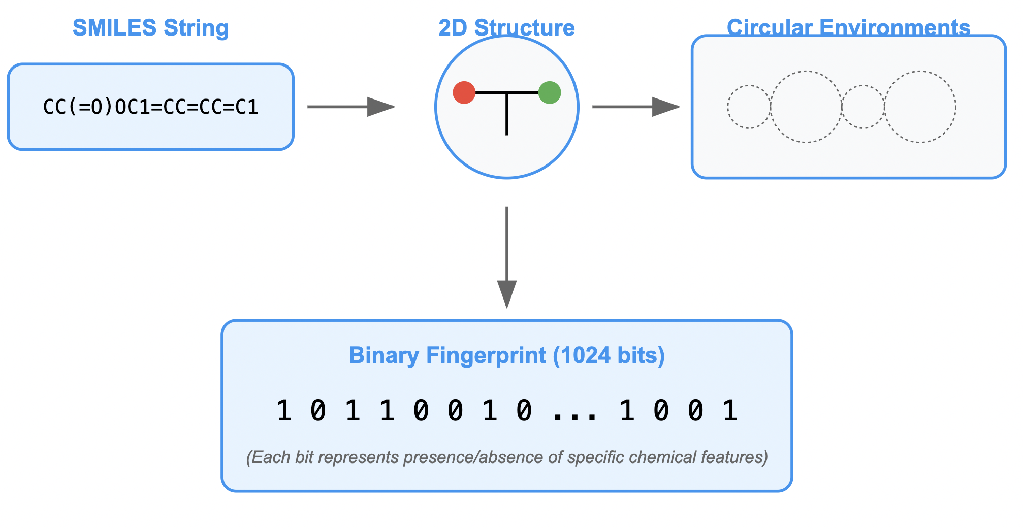
Figure: SMILES to Molecular Fingerprints Conversion Process
Step 4: Split Data into Training and Testing Sets
To evaluate the model, we need to split the data into training and testing sets. The train_test_split function from scikit-learn will handle this. We’ll use 80% of the data for training and 20% for testing.
from sklearn.model_selection import train_test_split

# Split data into train and test sets (80% training, 20% testing)
X_train, X_test, y_train, y_test = train_test_split(X, y, test_size=0.2, random_state=42)
The diagram below provides a visual representation of what this code does:
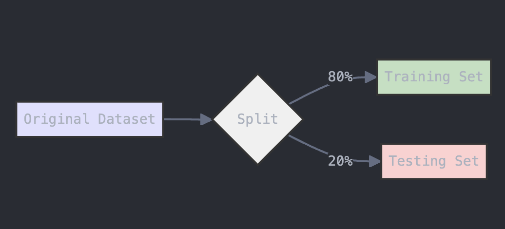
Figure: Data Splitting Process for Training and Testing
Step 5: Train the Random Forest Model
We’ll use the RandomForestClassifier from scikit-learn to build the model. A Random Forest is an ensemble method that uses multiple decision trees to make predictions. The more trees (n_estimators) we use, the more robust the model will be, but the longer the model will take to run. For the most part, n_estimators is set to 100 in most versions of scikit-learn. However, for more complex datasets, higher values like 500 or 1000 may improve performance.
from sklearn.ensemble import RandomForestClassifier

# Train a Random Forest classifier
rf_model = RandomForestClassifier(n_estimators=100, random_state=42)
rf_model.fit(X_train, y_train)
The diagram below provides a visual explanation of what is going on here:
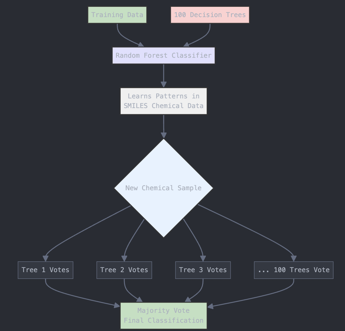
Figure: Random Forest Algorithm Structure
Step 6: Evaluate the Model
After training the model, we use the test data to check how well it performs. We measure its accuracy and also look at a classification report, which includes precision, recall, and F1 score.
Accuracy is the simplest metric: it tells us the percentage of all predictions the model got right — both permeable and non-permeable molecules.
Precision tells us how trustworthy the model’s positive (BBBP+) predictions are.
If the model predicts that a molecule can penetrate the blood-brain barrier, precision answers: Out of those predictions, how many were actually correct?
High precision means the model doesn’t make a lot of false positive mistakes — that is, it doesn’t often say a molecule can penetrate when it really can’t.
👉 Think of precision as: “When the model says yes, how often is it right?”
Recall tells us how good the model is at finding all the real positive cases.
In our BBBP example: out of all the molecules that actually can penetrate the blood-brain barrier, recall measures how many the model successfully identified.
High recall means the model finds most of the real positive cases and doesn’t miss many.
👉 Think of recall as: “How many of the true ‘yes’ molecules did the model catch?”
F1 score is a single number that balances precision and recall.
Sometimes a model may have high precision but low recall (it only predicts yes when very sure), or high recall but low precision (it predicts yes a lot, including mistakes).
The F1 score combines both precision and recall into one metric so we can judge overall performance when both are important.
👉 F1 is especially useful when the dataset is imbalanced — for example, if there are many more molecules that don’t cross the blood-brain barrier than those that do — because just looking at accuracy can be misleading in that case.
from sklearn.metrics import accuracy_score, classification_report

# Predictions on the test set
y_pred = rf_model.predict(X_test)

# Evaluate accuracy and performance
accuracy = accuracy_score(y_test, y_pred)
print("Accuracy:", accuracy)
print("Classification Report:", classification_report(y_test, y_pred))
Step 8: Visualizing Example Decision Trees
Although a Random Forest typically contains many decision trees, it is often helpful to visualize a few individual trees to gain intuition about how the model makes decisions.
In this section, we visualize three representative decision trees from the trained Random Forest. To keep the figures readable, only the top three levels of each tree are shown.
Step 8.1: Visualizing Individual Trees
Each internal node splits on a Morgan fingerprint bit (e.g., bit_919).
The condition bit_k <= 0.5 means the bit is absent (0) vs. present (1).
To keep the figure readable, we display only the first 3 levels of each tree.
import matplotlib.pyplot as plt
from sklearn.tree import plot_tree

# 1. Automatically determine fingerprint length based on the training data shape
n_bits = X_train.shape[1]
# Generate generic feature names (e.g., bit_0, bit_1, ...)
feature_names = [f"bit_{i}" for i in range(n_bits)]
# Define labels for the target classes
class_names = ["Non-Permeable (0)", "Permeable (1)"]

# 2. Select specific tree indices from the Random Forest to visualize
# Using [0, 1] will visualize the first and second trees
selected_tree_ids = [0, 1]

# Set the maximum depth to display; 2 or 3 is best to prevent the plot from being too crowded
PLOT_MAX_DEPTH = 2

for tid in selected_tree_ids:
    # Initialize a figure with high DPI for better text readability
    fig, ax = plt.subplots(figsize=(20, 10), dpi=100)

    # Plot the decision tree logic
    plot_tree(
        rf_model.estimators_[tid], # Select the specific tree estimator
        max_depth=PLOT_MAX_DEPTH,   # Limit depth to keep the visual clean
        feature_names=feature_names,
        class_names=class_names,
        filled=True,                # Color nodes by majority class
        rounded=True,               # Use rounded boxes for aesthetics
        proportion=True,            # Show percentages instead of raw sample counts
        impurity=False,             # Hide impurity metrics to reduce clutter
        fontsize=12,
        ax=ax                       # Explicitly assign to current axis
    )

    # Add a title identifying the specific tree number
    ax.set_title(f"Random Forest - Tree #{tid}", fontsize=15)

    # Render the plot for each iteration
    plt.show()
Step 8.2: Example Trees
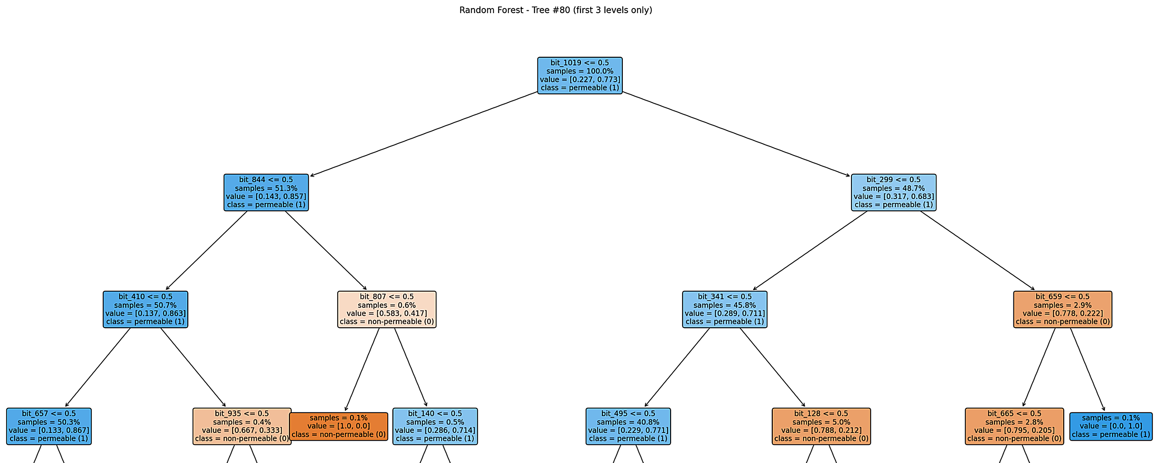
Figure: Example decision tree (Tree #80).
This tree is globally biased toward predicting permeability, while a few specific fingerprint bits create small branches that strongly indicate non-permeability.
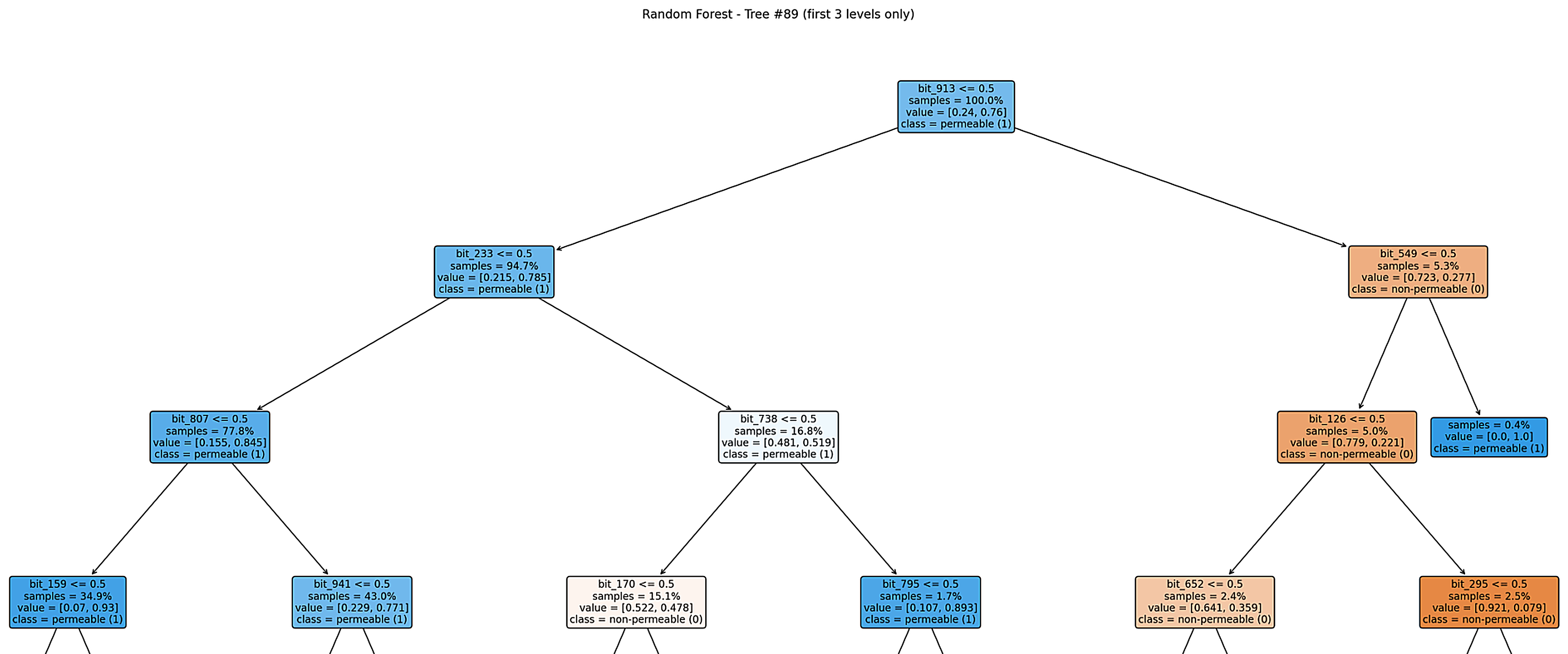
Figure: Example decision tree (Tree #89).
Most samples follow a permeable path, but a small subset is quickly classified as non-permeable once certain fingerprint bits are present.
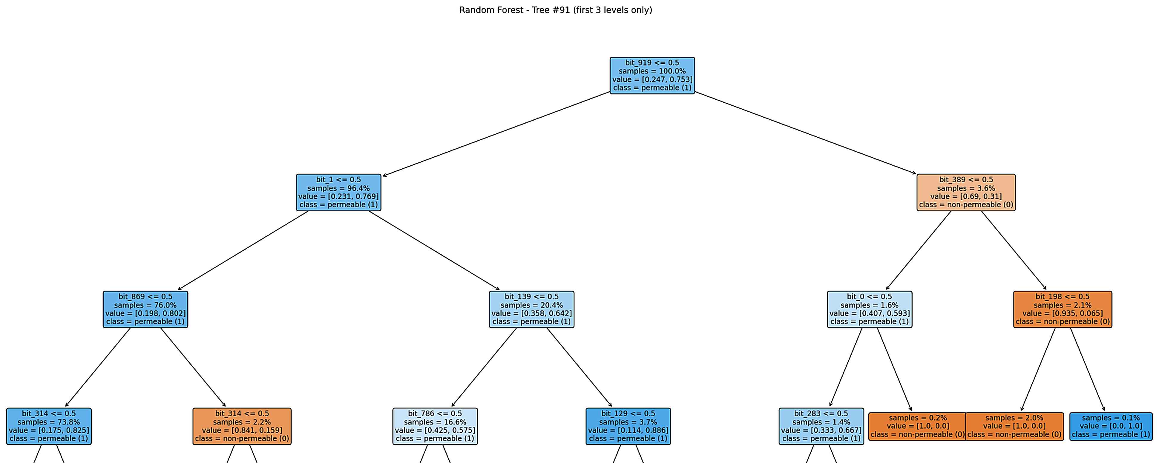
Figure: Example decision tree (Tree #91).
The tree refines predictions within the permeable class while reserving a few high-confidence branches for non-permeable compounds.
These visualizations illustrate how individual decision trees in a Random Forest make predictions based on molecular fingerprint features, while the ensemble combines many such trees to achieve strong overall performance.
Model Performance and Parameters
- Accuracy: The proportion of correctly predicted instances out of all instances.
- Classification Report: Provides additional metrics like precision, recall, and F1 score.
In this case, we achieved an accuracy score of ~87%.
Key Hyperparameters:
- n_estimators: The number of trees in the Random Forest. More trees generally lead to better performance but also require more computational resources.
- test_size: The proportion of data used for testing. A larger test size gives a more reliable evaluation but reduces the amount of data used for training.
- random_state: Ensures reproducibility by initializing the random number generator to a fixed seed.
Conclusion
This guide demonstrated how to implement a Random Forest model to predict the Blood–Brain Barrier Permeability (BBBP) using the BBBP dataset. By converting SMILES strings to molecular fingerprints and using a Random Forest classifier, we were able to achieve an accuracy score of around 87%.
Adjusting parameters like the number of trees (n_estimators) or the split ratio (test_size) can help improve the model’s performance. Feel free to experiment with these parameters and explore other machine learning models for this task!
3.1.4 Approaching Random Forest Problems
When tackling a classification or regression problem using the Random Forest algorithm, a systematic approach can enhance your chances of success. Here’s a step-by-step guide to effectively solve any Random Forest problem:
-
Understand the Problem Domain: Begin by thoroughly understanding the problem you are addressing. Identify the nature of the data and the specific goal—whether it’s classification (e.g., predicting categories) or regression (e.g., predicting continuous values). Familiarize yourself with the dataset, including the features (independent variables) and the target variable (dependent variable).
-
Data Collection and Preprocessing: Gather the relevant dataset and perform necessary preprocessing steps. This may include handling missing values, encoding categorical variables, normalizing or standardizing numerical features, and removing any outliers. Proper data cleaning ensures that the model learns from quality data.
-
Exploratory Data Analysis (EDA): Conduct an exploratory data analysis to understand the underlying patterns, distributions, and relationships within the data. Visualizations, such as scatter plots, histograms, and correlation matrices, can provide insights that inform feature selection and model tuning.
-
Feature Selection and Engineering: Identify the most relevant features for the model. This can be achieved through domain knowledge, statistical tests, or feature importance metrics from preliminary models. Consider creating new features through feature engineering to enhance model performance.
-
Model Training and Parameter Tuning: Split the dataset into training and testing sets, typically using an 80-20 or 70-30 ratio. Train the Random Forest model using the training data, adjusting parameters such as the number of trees (
n_estimators), the maximum depth of the trees (max_depth), and the minimum number of samples required to split an internal node (min_samples_split). Utilize techniques like grid search or random search to find the optimal hyperparameters. -
Model Evaluation: Once trained, evaluate the model’s performance on the test set using appropriate metrics. For classification problems, metrics such as accuracy, precision, recall, F1 score, and ROC-AUC are valuable. For regression tasks, consider metrics like mean absolute error (MAE), mean squared error (MSE), and R-squared.
-
Interpretation and Insights: Analyze the model’s predictions and feature importance to derive actionable insights. Understanding which features contribute most to the model can guide decision-making and further improvements in the model or data collection.
-
Iterate and Improve: Based on the evaluation results, revisit the previous steps to refine your model. This may involve further feature engineering, collecting more data, or experimenting with different algorithms alongside Random Forest to compare performance.
-
Deployment: Once satisfied with the model’s performance, prepare it for deployment. Ensure the model can process incoming data and make predictions in a real-world setting, and consider implementing monitoring tools to track its performance over time.
By following this structured approach, practitioners can effectively leverage the Random Forest algorithm to solve a wide variety of problems, ensuring thorough analysis, accurate predictions, and actionable insights.
3.1.5 Strengths and Weaknesses of Random Forest
Strengths:
-
Robustness: Random Forests are less prone to overfitting compared to individual decision trees, making them more reliable for new data.
-
Versatility: They can handle both classification and regression tasks effectively.
-
Feature Importance: Random Forests provide insights into the significance of each feature in making predictions.
Weaknesses:
-
Complexity: The model can become complex, making it less interpretable than single decision trees.
-
Resource Intensive: Training a large number of trees can require significant computational resources and time.
-
Slower Predictions: While individual trees are quick to predict, aggregating predictions from multiple trees can slow down the prediction process.
Section 3.1 – Quiz Questions
1) Factual Questions
Question 1
What is the primary reason a Decision Tree might perform very well on training data but poorly on new, unseen data?
A. Underfitting
B. Data leakage
C. Overfitting
D. Regularization
▶ Click to show answer
Correct Answer: C▶ Click to show explanation
Explanation: Decision Trees can easily overfit the training data by creating very complex trees that capture noise instead of general patterns. This hurts their performance on unseen data.Question 2
In a Decision Tree, what do the internal nodes represent?
A. Possible outcomes
B. Splitting based on a feature
C. Aggregation of multiple trees
D. Random subsets of data
▶ Click to show answer
Correct Answer: B▶ Click to show explanation
Explanation: Internal nodes represent decision points where the dataset is split based on the value of a specific feature (e.g., "Is the fruit color red or orange?").Question 3
Which of the following best explains the Random Forest algorithm?
A. A single complex decision tree trained on all the data
B. Many decision trees trained on identical data to improve depth
C. Many decision trees trained on random subsets of the data and features
D. A clustering algorithm that separates data into groups
▶ Click to show answer
Correct Answer: C▶ Click to show explanation
Explanation: Random Forests use bagging to train multiple decision trees on different random subsets of the data and different random subsets of features, making the ensemble more robust.Question 4
When training a Random Forest for a classification task, how is the final prediction made?
A. By taking the median of the outputs
B. By taking the average of probability outputs
C. By majority vote among trees’ predictions
D. By selecting the tree with the best accuracy
▶ Click to show answer
Correct Answer: C▶ Click to show explanation
Explanation: For classification problems, the Random Forest algorithm uses majority voting — the class most predicted by the individual trees becomes the final prediction.2) Conceptual Questions
Question 5
You are given a dataset containing information about chemical compounds, with many categorical features (such as “molecular class” or “bond type”).
Would using a Random Forest model be appropriate for this dataset?
A. No, Random Forests cannot handle categorical data.
B. Yes, Random Forests can naturally handle datasets with categorical variables after encoding.
C. No, Random Forests only work on images.
D. Yes, but only if the dataset has no missing values.
▶ Click to show answer
Correct Answer: B▶ Click to show explanation
Explanation: Random Forests can handle categorical data after simple preprocessing, such as label encoding or one-hot encoding. They are robust to different feature types, including numerical and categorical.Question 6
Suppose you have your molecule fingerprints stored in variables X and your labels (0 or 1 for BBBP) stored in y.
Which of the following correctly splits the data into 80% training and 20% testing sets?
A.
X_train, X_test, y_train, y_test = train_test_split(X, y, train_size=0.2, random_state=42)
B.
X_train, X_test, y_train, y_test = train_test_split(X, y, test_size=0.2, random_state=42)
C.
X_train, X_test = train_test_split(X, y, test_size=0.8, random_state=42)
D.
X_train, y_train, X_test, y_test = train_test_split(X, y, test_size=0.2, random_state=42)
▶ Click to show answer
Correct Answer: B▶ Click to show explanation
Explanation: In Random Forest modeling, we use train_test_split from sklearn.model_selection. test_size=0.2 reserves 20% of the data for testing, leaving 80% for training. The function returns train features, test features, train labels, and test labels — in that exact order: X_train, X_test, y_train, y_test = train_test_split(X, y, test_size=0.2, random_state=42) A, C, and D are wrong because... (A) reverses train and test sizing. (C) mistakenly sets test_size=0.8 (which would leave only 20% for training — wrong). (D) messes up the return order (train features and labels must come first).▶ Show Solution Code
from sklearn.model_selection import train_test_split

X_train, X_test, y_train, y_test = train_test_split(X, y, test_size=0.2, random_state=42)