3-C. Machine Learning Models
3.3 Graph Neural Networks
Completed and Compiled Code (3.3.1–3.3.3): Click Here
A Graph Neural Network (GNN) is built for graph-structured data. Nodes carry features, edges carry relationships, and learning proceeds by passing messages along edges, updating node states, and then reading out a graph-level vector for a downstream task.
Structure. Layers alternate between (i) message passing—neighbors send transformed signals along edges—and (ii) state updates—each node revises its embedding with a nonlinear function. Stacking (k) layers exposes a node to its (k)-hop neighborhood. A final readout/pooling (e.g., sum/mean) aggregates node embeddings into a fixed-length molecular representation.
Functioning. In molecular graphs, atoms = nodes and bonds = edges. Messages combine atom features with bond features, propagate to destination atoms, and are transformed (e.g., by MLPs or GRUs). After several layers, each atom’s embedding reflects its local chemical context (hybridization, aromaticity, ring membership, nearby heteroatoms).
Learning. Training minimizes a task loss (e.g., BCEWithLogits for classification) with gradient descent. Gradients flow through the graph topology, tuning how atoms attend to their neighbors and how the pooled representation supports the final prediction.
Roadmap.
3.3.1 looks at OGB-MOLHIV, the dataset and official split, and builds loaders with basic EDA.
3.3.2 implements an edge-aware MPNN (NNConv + GRU) and reads the curves/ROC.
3.3.3 compares GCN and MPNN on the same split and discusses the outcomes.
3.3.1 From Descriptors to Molecular Graphs: OGB-MOLHIV at a Glance
Why start here. Descriptor-only QSAR can flatten connectivity; a molecular GNN keeps the who-is-bonded-to-whom information. The OGB-MOLHIV benchmark (Hu et al., 2020) provides graph data (atoms, bonds) with an anti-HIV activity label and an official train/valid/test split—ideal for a clean, reproducible pipeline.
| Key Functions and Concepts (Data Layer) | ||
|---|---|---|
|
PygGraphPropPredDataset OGB–PyG dataset wrapper Auto-download + official split |
DataLoader (PyG) Mini-batches of graphs Collates Data objects into DataBatch |
DataBatch fieldsx, edge_index, edge_attr, yAtoms (9-dim), bonds (3-dim), labels |
3.3.1-A Load the dataset and the official split
What this cell does. Imports minimal packages, downloads/loads ogbg-molhiv, and fetches the official indices for train/valid/test.
# Minimal imports
import numpy as np, matplotlib.pyplot as plt, torch
from ogb.graphproppred import PygGraphPropPredDataset
from torch_geometric.loader import DataLoader

# Load + split
dataset = PygGraphPropPredDataset(name="ogbg-molhiv")
split = dataset.get_idx_split()
train_set, valid_set, test_set = dataset[split["train"]], dataset[split["valid"]], dataset[split["test"]]

print(dataset)
print(f"Graphs: total={len(dataset)} | train/valid/test = {len(train_set)}/{len(valid_set)}/{len(test_set)}")
Results
PygGraphPropPredDataset(41127)Graphs: total=41127 | train/valid/test = 32901/4113/4113
This confirms the canonical OGB split we use throughout.
3.3.1-B Quick EDA (label skew, nodes/edges per graph)
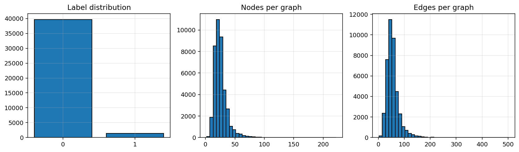
What this cell does. Builds three histograms: label distribution, atoms per molecule, and bonds per molecule—so we know the class balance and a reasonable message-passing depth.
labels = dataset.data.y.view(-1).cpu().numpy()
num_nodes = [g.num_nodes for g in dataset]
num_edges = [g.num_edges for g in dataset]

fig, axs = plt.subplots(1, 3, figsize=(12, 3.6), dpi=140)
axs[0].hist(labels, bins=[-0.5,0.5,1.5], rwidth=0.8, edgecolor="black"); axs[0].set_xticks([0,1])
axs[0].set_title("Label distribution"); axs[0].grid(alpha=0.3)
axs[1].hist(num_nodes, bins=40, edgecolor="black"); axs[1].set_title("Nodes per graph"); axs[1].grid(alpha=0.3)
axs[2].hist(num_edges, bins=40, edgecolor="black"); axs[2].set_title("Edges per graph"); axs[2].grid(alpha=0.3)
plt.tight_layout(); plt.show()
How to read it. Labels are heavily imbalanced (positives ≪ negatives), so ROC-AUC is a better main metric than accuracy, and class-weighted BCE is advisable. Graph sizes are mostly in the tens of atoms/bonds, so 2–4 message-passing layers are a reasonable starting point.
3.3.1-C DataLoaders + a batch sanity check
What this cell does. Creates loaders and prints one training batch to confirm feature shapes (we will reuse the loaders later).
train_loader = DataLoader(train_set, batch_size=64, shuffle=True)
valid_loader = DataLoader(valid_set, batch_size=256, shuffle=False)
test_loader  = DataLoader(test_set,  batch_size=256, shuffle=False)

batch = next(iter(train_loader))
print(batch)
print("num_graphs:", batch.num_graphs,
      "| node_feat_dim:", batch.x.size(-1),
      "| edge_feat_dim:", batch.edge_attr.size(-1),
      "| y shape:", tuple(batch.y.view(-1).shape))
Results
DataBatch(edge_index=[2, 3640], edge_attr=[3640, 3], x=[1711, 9], y=[64, 1], …)num_graphs: 64 | node_feat_dim: 9 | edge_feat_dim: 3 | y shape: (64,)
This confirms the exact input dimensions we connect to the models in §3.3.2 and §3.3.3.
3.3.2 Message Passing as Chemical Reasoning (NNConv–GRU MPNN)
The Message Passing Neural Network (MPNN) (Gilmer et al., 2017) is a family of GNNs designed to learn directly from molecular graphs. Each atom updates its representation by aggregating messages from its neighboring atoms through bonds. In our implementation, bond features determine how messages are weighted, and a Gated Recurrent Unit (GRU) stabilizes multi-step updates.
Goal. Build and train an edge-aware MPNN (using NNConv + GRU) for molecular property prediction on ogbg-molhiv, record training dynamics, and evaluate the ROC-AUC on the held-out test set.
| Key Functions and Concepts (MPNN) | |||
|---|---|---|---|
|
NNConv Edge-conditioned convolution Uses bond features to parameterize message filters |
EdgeNet MLP for edge feature transformation Maps edge attributes → filter matrices |
GRU Gated recurrent unit Controls information flow across layers |
global_add_pool Readout layer Aggregates atomic embeddings → molecule representation |
3.3.2-A Reproducibility, device, and class weight
This first cell ensures consistent runs and builds loaders for the model.
Because the MOLHIV dataset is imbalanced, we compute a positive-class weight for use in BCEWithLogitsLoss.
import random, numpy as np, torch
from ogb.graphproppred import PygGraphPropPredDataset
from torch_geometric.loader import DataLoader

# Fix randomness for reproducibility
def set_seed(s=1):
    random.seed(s); np.random.seed(s)
    torch.manual_seed(s); torch.cuda.manual_seed_all(s)
set_seed(1)

# Select device (GPU if available)
device = torch.device("cuda" if torch.cuda.is_available() else "cpu")

# Load dataset and official splits
dataset = PygGraphPropPredDataset(name="ogbg-molhiv")
split = dataset.get_idx_split()
train_loader = DataLoader(dataset[split["train"]], batch_size=64, shuffle=True)
valid_loader = DataLoader(dataset[split["valid"]], batch_size=256, shuffle=False)
test_loader  = DataLoader(dataset[split["test"]],  batch_size=256, shuffle=False)

# Compute class weight (for imbalance)
train_y = dataset[split["train"]].y.view(-1).cpu().numpy()
pos_weight = torch.tensor([(train_y==0).sum()/(train_y==1).sum()], dtype=torch.float, device=device)

D_x, D_e = dataset.num_node_features, dataset.num_edge_features
Explanation.
This setup guarantees that experiments are repeatable.
pos_weight > 1 tells the loss function to assign higher penalty to misclassified positive samples.
3.3.2-B Define the model: EdgeNet + NNConv + GRU
This section builds the network architecture. Each message-passing layer applies an edge-specific linear transformation followed by a GRU update and dropout for regularization.
import torch.nn as nn, torch.nn.functional as F
from torch_geometric.nn import NNConv, global_add_pool

class EdgeNet(nn.Module):
    """Small MLP that transforms edge features into NNConv filters."""
    def __init__(self, edge_in, hidden):
        super().__init__()
        self.net = nn.Sequential(
            nn.Linear(edge_in, hidden*hidden),
            nn.ReLU(),
            nn.Linear(hidden*hidden, hidden*hidden)
        )
        self.hidden = hidden

    def forward(self, e):  # e: [E, edge_in]
        return self.net(e)  # Output: [E, hidden*hidden]


class MPNN(nn.Module):
    """Message Passing Neural Network with edge-conditioned messages."""
    def __init__(self, node_in, edge_in, hidden=128, layers=3, dropout=0.2):
        super().__init__()
        self.embed = nn.Linear(node_in, hidden)
        self.edge_net = EdgeNet(edge_in, hidden)
        self.convs = nn.ModuleList([
            NNConv(hidden, hidden, self.edge_net, aggr='add') for _ in range(layers)
        ])
        self.gru = nn.GRU(hidden, hidden)
        self.dropout = dropout
        self.readout = nn.Linear(hidden, 1)

    def forward(self, data):
        x, edge_index, edge_attr, batch = data.x.float(), data.edge_index, data.edge_attr, data.batch
        # Safety guard: ensure bond features are floats
        if edge_attr is None:
            edge_attr = torch.zeros((edge_index.size(1), D_e), dtype=torch.float, device=x.device)
        else:
            edge_attr = edge_attr.float()

        # 1) Embed atom features
        x = self.embed(x)
        h = x.unsqueeze(0)

        # 2) Perform message passing and gated update
        for conv in self.convs:
            m = F.relu(conv(x, edge_index, edge_attr))
            m = F.dropout(m, p=self.dropout, training=self.training).unsqueeze(0)
            out, h = self.gru(m, h)
            x = out.squeeze(0)

        # 3) Aggregate to graph-level representation
        g = global_add_pool(x, batch)

        # 4) Linear readout → logit
        return self.readout(g).view(-1)
Explanation.
EdgeNetmaps 3-dimensional bond descriptors to layer-specific filters.NNConvuses those filters to compute neighbor messages.GRUdecides how much new information to incorporate versus retain from previous states.global_add_poolsums over all atoms to yield a molecule-level vector.
3.3.2-C Training, validation (AUC), and testing (ROC)
The training loop minimizes BCEWithLogitsLoss, monitors AUC on the validation split, and restores the best weights before evaluating on the test set.
from sklearn.metrics import roc_auc_score, roc_curve
import matplotlib.pyplot as plt, numpy as np
def train_epoch(model, loader, opt, crit, clip=2.0):
"""Single epoch of training."""
model.train(); total, n = 0.0, 0
for data in loader:
data = data.to(device)
y = data.y.view(-1).float()
opt.zero_grad()
logits = model(data)
loss = crit(logits, y)
loss.backward()
nn.utils.clip_grad_norm_(model.parameters(), clip)
opt.step()
total += loss.item() * y.numel(); n += y.numel()
return total / n
@torch.no_grad()
def eval_auc(model, loader):
"""Compute ROC-AUC on a loader."""
model.eval(); y_true, y_prob = [], []
for data in loader:
data = data.to(device)
prob = torch.sigmoid(model(data)).cpu().numpy()
y_true.append(data.y.view(-1).cpu().numpy())
y_prob.append(prob)
y_true = np.concatenate(y_true); y_prob = np.concatenate(y_prob)
auc = roc_auc_score(y_true, y_prob)
fpr, tpr, _ = roc_curve(y_true, y_prob)
return auc, (fpr, tpr)
# Initialize model, optimizer, and loss
model = MPNN(D_x, D_e, hidden=128, layers=3, dropout=0.2).to(device)
opt = torch.optim.Adam(model.parameters(), lr=1e-3, weight_decay=1e-5)
crit = nn.BCEWithLogitsLoss(pos_weight=pos_weight)
best_val, best_state = -1.0, None
train_curve, val_curve = [], []
# Train for 20 epochs
for ep in range(1, 21):
tr = train_epoch(model, train_loader, opt, crit)
va, _ = eval_auc(model, valid_loader)
train_curve.append(tr); val_curve.append(va)
if va > best_val:
best_val = va
best_state = {k: v.cpu() for k, v in model.state_dict().items()}
print(f"Epoch {ep:02d} | train {tr:.4f} | valid AUC {va:.4f}")
# Restore best checkpoint and test
model.load_state_dict({k: v.to(device) for k, v in best_state.items()})
test_auc, (fpr, tpr) = eval_auc(model, test_loader)
print(f"[MPNN] Best valid AUC = {best_val:.4f} | Test AUC = {test_auc:.4f}")
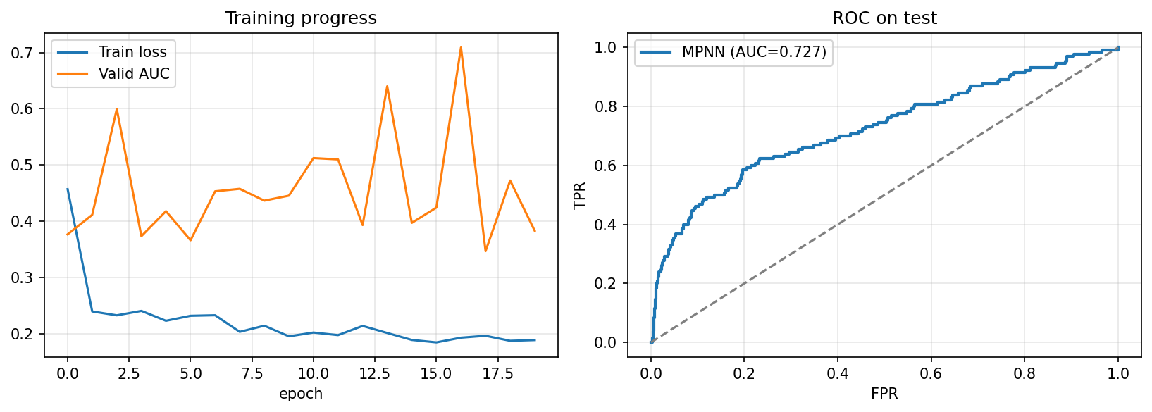
# Plot results
fig, axs = plt.subplots(1, 2, figsize=(11, 4), dpi=150)
axs[0].plot(train_curve, label="Train loss")
axs[0].plot(val_curve, label="Valid AUC")
axs[0].set_title("Training progress")
axs[0].set_xlabel("Epoch")
axs[0].grid(alpha=0.3)
axs[0].legend()
axs[1].plot(fpr, tpr, lw=2, label=f"MPNN (AUC={test_auc:.3f})")
axs[1].plot([0,1],[0,1],"--",color="gray")
axs[1].set_xlabel("False Positive Rate")
axs[1].set_ylabel("True Positive Rate")
axs[1].set_title("ROC on test")
axs[1].grid(alpha=0.3)
axs[1].legend()
plt.tight_layout(); plt.show()
Training Log (excerpt)
Epoch 17 … valid AUC 0.7089→ bestTest AUC = 0.7268
Interpretation.
- Training loss decreases smoothly to ≈ 0.18.
- Validation AUC fluctuates between 0.35 – 0.70 due to class imbalance and small batch effects, peaking around 0.71.
- The best test AUC ≈ 0.73 shows that the model captures useful substructural information even in a compact configuration.
- The oscillations are typical for imbalanced molecular classification tasks; early stopping at the validation peak prevents overfitting.
References (for §3.3 & §3.3.1 §3.3.2)
- Fey, M., & Lenssen, J. E. (2019). PyTorch Geometric.
- Hu, W. et al. (2020). Open Graph Benchmark.
- Wu, Z. et al. (2018). MoleculeNet.
3.3.3 Same Split, Two Architectures: GCN vs Edge-aware MPNN
We now place two graph architectures side by side on the same OGB-MOLHIV split and with the same evaluation metric (ROC-AUC):
- GCN (Kipf & Welling, 2017): neighborhood aggregation without an edge MLP; all bonds contribute uniformly.
- MPNN (NNConv + GRU): messages are edge-conditioned by bond features; a GRU stabilizes multi-step updates.
The point is to contrast how the two formulations behave under an identical training recipe, not to assume one is inherently superior.
| Key Functions and Concepts (Comparison) | |||
|---|---|---|---|
|
GCNConv Graph convolution (no bond MLP) Uniform treatment of bonds during aggregation |
NNConv Edge-conditioned convolution Bond features → per-edge filters |
GRU Gated update across layers Stabilizes multi-step message passing |
ROC-AUC Ranking under class imbalance Threshold-free comparison |
Note. This subsection reuses the loaders and
pos_weightfrom §3.3.2 (3.3.2-A). If you run cells independently, execute §3.3.1 and §3.3.2-A first.
3.3.3-A Define the two architectures succinctly
What this cell does. Implements a compact GCN baseline and the NNConv + GRU MPNN; both end with global_add_pool and a linear head that outputs a logit per molecule.
import torch.nn as nn, torch.nn.functional as F
from torch_geometric.nn import GCNConv, NNConv, global_add_pool

class GCN_Baseline(nn.Module):
    def __init__(self, in_dim, hidden=128, layers=3, dropout=0.2):
        super().__init__()
        self.embed = nn.Linear(in_dim, hidden)
        self.convs = nn.ModuleList([GCNConv(hidden, hidden) for _ in range(layers)])
        self.drop  = dropout
        self.out   = nn.Linear(hidden, 1)
    def forward(self, data):
        x, edge_index, batch = data.x.float(), data.edge_index, data.batch
        x = self.embed(x)
        for conv in self.convs:
            x = F.relu(conv(x, edge_index))
            x = F.dropout(x, p=self.drop, training=self.training)
        g = global_add_pool(x, batch)
        return self.out(g).view(-1)

class EdgeNet(nn.Module):
    def __init__(self, edge_in, hidden):
        super().__init__()
        self.net = nn.Sequential(
            nn.Linear(edge_in, hidden*hidden), nn.ReLU(),
            nn.Linear(hidden*hidden, hidden*hidden)
        ); self.hidden = hidden
    def forward(self, e): return self.net(e)

class MPNN_NNConv(nn.Module):
    def __init__(self, node_in, edge_in, hidden=128, layers=3, dropout=0.2):
        super().__init__()
        self.embed   = nn.Linear(node_in, hidden)
        self.edge_net= EdgeNet(edge_in, hidden)
        self.convs   = nn.ModuleList([NNConv(hidden, hidden, self.edge_net, aggr='add') for _ in range(layers)])
        self.gru     = nn.GRU(hidden, hidden)
        self.drop    = dropout
        self.out     = nn.Linear(hidden, 1)
    def forward(self, data):
        x, edge_index, edge_attr, batch = data.x.float(), data.edge_index, data.edge_attr, data.batch
        edge_attr = edge_attr.float() if edge_attr is not None else torch.zeros((edge_index.size(1), D_e), device=x.device)
        x = self.embed(x); h = x.unsqueeze(0)
        for conv in self.convs:
            m = F.relu(conv(x, edge_index, edge_attr))
            m = F.dropout(m, p=self.drop, training=self.training).unsqueeze(0)
            out, h = self.gru(m, h); x = out.squeeze(0)
        g = global_add_pool(x, batch)
        return self.out(g).view(-1)
3.3.3-B Shared training/evaluation routine
What this cell does. Trains either model with the same loop and hyperparameters, selects the best validation AUC checkpoint, and reports test AUC and ROC.
from sklearn.metrics import roc_auc_score, roc_curve
import numpy as np, torch

def train_and_select(model, tag, train_loader, valid_loader, test_loader, pos_weight=None, epochs=15, lr=1e-3):
    device = next(model.parameters()).device
    opt  = torch.optim.Adam(model.parameters(), lr=lr, weight_decay=1e-5)
    crit = nn.BCEWithLogitsLoss(pos_weight=pos_weight)
    best_val, best = -1.0, None

    for ep in range(1, epochs+1):
        # Train one epoch
        model.train(); tot, n = 0.0, 0
        for data in train_loader:
            data = data.to(device); y = data.y.view(-1).float()
            opt.zero_grad(); loss = crit(model(data), y); loss.backward()
            nn.utils.clip_grad_norm_(model.parameters(), 2.0); opt.step()
            tot += loss.item() * y.numel(); n += y.numel()

        # Validate
        model.eval(); y_true, y_prob = [], []
        with torch.no_grad():
            for data in valid_loader:
                data = data.to(device)
                p = torch.sigmoid(model(data)).cpu().numpy()
                y_true.append(data.y.view(-1).cpu().numpy()); y_prob.append(p)
        y_true = np.concatenate(y_true); y_prob = np.concatenate(y_prob)
        val_auc = roc_auc_score(y_true, y_prob)
        print(f"[{tag}] epoch {ep:02d} | train {tot/n:.4f} | valid AUC {val_auc:.4f}")

        if val_auc > best_val:
            best_val = val_auc
            best = {k: v.cpu() for k, v in model.state_dict().items()}

    # Test with best checkpoint
    model.load_state_dict({k: v.to(device) for k, v in best.items()})
    model.eval(); y_true, y_prob = [], []
    with torch.no_grad():
        for data in test_loader:
            data = data.to(device)
            p = torch.sigmoid(model(data)).cpu().numpy()
            y_true.append(data.y.view(-1).cpu().numpy()); y_prob.append(p)
    y_true = np.concatenate(y_true); y_prob = np.concatenate(y_prob)
    test_auc = roc_auc_score(y_true, y_prob)
    fpr, tpr, _ = roc_curve(y_true, y_prob)
    print(f"[{tag}] BEST valid AUC {best_val:.4f} | TEST AUC {test_auc:.4f}")
    return test_auc, (fpr, tpr)
3.3.3-C Run both models and visualize
What this cell does. Instantiates GCN and MPNN, runs the shared routine for 15 epochs, and produces ROC curves plus a bar chart of the two AUCs.
import matplotlib.pyplot as plt

gcn  = GCN_Baseline(D_x).to(device)
mpnn = MPNN_NNConv(D_x, D_e).to(device)

gcn_auc, (gcn_fpr, gcn_tpr)   = train_and_select(gcn,  "GCN",  train_loader, valid_loader, test_loader, pos_weight, epochs=15)
mpn_auc, (mpn_fpr, mpn_tpr)   = train_and_select(mpnn, "MPNN", train_loader, valid_loader, test_loader, pos_weight, epochs=15)

# Plot ROC and AUC bars
fig, ax = plt.subplots(1, 2, figsize=(11, 4), dpi=150)
ax[0].plot(gcn_fpr, gcn_tpr, lw=2, label=f"GCN (AUC={gcn_auc:.3f})")
ax[0].plot(mpn_fpr, mpn_tpr, lw=2, label=f"MPNN/NNConv (AUC={mpn_auc:.3f})")
ax[0].plot([0,1],[0,1],"--",color="gray"); ax[0].set_xlabel("FPR"); ax[0].set_ylabel("TPR")
ax[0].set_title("ROC on test"); ax[0].grid(alpha=0.3); ax[0].legend()

ax[1].bar(["GCN","MPNN"], [gcn_auc, mpn_auc], edgecolor="black", alpha=0.9)
for x, v in zip(["GCN","MPNN"], [gcn_auc, mpn_auc]):
    ax[1].text(x, v+0.01, f"{v:.3f}", ha="center", va="bottom")
ax[1].set_ylim(0, 1.05); ax[1].set_ylabel("AUC"); ax[1].set_title("AUC comparison")
ax[1].grid(axis="y", alpha=0.3)
plt.tight_layout(); plt.show()
Recorded results GCN
[GCN] … BEST valid AUC 0.7212 | TEST AUC 0.6640MPNN (quick comparison recipe)[MPNN] … BEST valid AUC 0.5505 | TEST AUC 0.5894
Figure
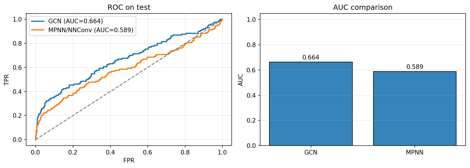
How to read these outcomes (with the logs)
- Under the shared 15-epoch recipe, the GCN run landed at test AUC ≈ 0.664, while the quick MPNN comparison run landed at ≈ 0.589.
- In §3.3.2, a separate MPNN run—same split but with early-stopping at the sharp validation peak and 20 epochs—reached test AUC ≈ 0.727.
- Together, these runs show how training choices (epoch budget, early-stopping point, class weighting, LR/scheduler) influence the two architectures differently. The comparison here is useful to see relative behavior under the same budget; §3.3.2 shows what the edge-aware model can achieve with a slightly longer/steadier training loop.
Optional dials to try (one at a time).
Epochs 30–40 for MPNN; LR (5\times 10^{-4}) for MPNN; hidden 256 (layers=3); ReduceLROnPlateau on validation AUC; keep weight_decay=1e-5, dropout=0.2.
References (for §3.3.3) Kipf & Welling, 2017 (GCN); Gilmer et al., 2017 (MPNN); Fey & Lenssen, 2019 (PyG); Hu et al., 2020 (OGB).
3.3.4 Challenges and Interpretability in GNNs
Completed and Compiled Code: Click Here
What We're Exploring: Fundamental Challenges in Graph Neural Networks
Why Study GNN Challenges?
- Over-smoothing: Why deeper isn't always better - node features become indistinguishable
- Interpretability: Understanding what the model learns - crucial for drug discovery
- Real Impact: These challenges affect whether GNNs can be trusted in production
What you'll learn: The fundamental limitations of GNNs and current solutions to overcome them
| Challenge | What Happens | Why It Matters | Solutions |
|---|---|---|---|
| Over-smoothing | Node features converge All atoms look the same |
Limits network depth Can't capture long-range interactions |
Residual connections Skip connections, normalization |
| Interpretability | Black box predictions Don't know why it predicts |
No trust in predictions Can't guide drug design |
Attention visualization Substructure explanations |
While GNNs have shown remarkable success in molecular property prediction, they face several fundamental challenges that limit their practical deployment. In this section, we’ll explore two critical issues: the over-smoothing phenomenon that limits network depth, and the interpretability challenge that makes it difficult to understand model predictions.
The Power of Depth vs. The Curse of Over-smoothing
In Graph Neural Networks (GNNs), adding more message-passing layers allows nodes (atoms) to gather information from increasingly distant parts of a graph (molecule). At first glance, it seems deeper networks should always perform better—after all, more layers mean more context. But in practice, there’s a major trade-off known as over-smoothing.
Understanding Over-smoothing
| Concept | Simple Explanation | Molecular Context |
|---|---|---|
| Message Passing | Atoms share info with neighbors | Like atoms "talking" through bonds |
| Receptive Field | How far information travels | k layers = k-hop neighborhood |
| Over-smoothing | All nodes become similar | Can't distinguish different atoms |
| Critical Depth | ~3-5 layers typically | Beyond this, performance drops |
What to Demonstrate
Before we jump into the code, here’s what it’s trying to show:
We want to measure how similar node embeddings become as we increase the number of GCN layers. If all node vectors become nearly identical after several layers, that means the model is losing resolution—different atoms can’t be distinguished anymore. This is called over-smoothing.
| Key Functions and Concepts | |||
|---|---|---|---|
|
GCNConv Graph convolution layer Aggregates neighbor features |
F.relu() Non-linear activation Adds expressiveness |
F.normalize() L2 normalization For cosine similarity |
torch.mm() Matrix multiplication Computes similarity matrix |
Functions and Concepts Used
-
GCNConv(fromtorch_geometric.nn): This is a standard Graph Convolutional Network (GCN) layer. It performs message passing by aggregating neighbor features and updating node embeddings. It normalizes messages by node degrees to prevent high-degree nodes from dominating. -
F.relu(): Applies a non-linear ReLU activation function after each GCN layer. This introduces non-linearity to the model, allowing it to learn more complex patterns. -
F.normalize(..., p=2, dim=1): This normalizes node embeddings to unit length (L2 norm), which is required for cosine similarity calculation. -
torch.mm(): Matrix multiplication is used here to compute the full cosine similarity matrix between normalized node embeddings. -
Cosine similarity: Measures how aligned two vectors are (value close to 1 means very similar). By averaging all pairwise cosine similarities, we can track whether the node representations are collapsing into the same vector.
Graph Construction
We use a 6-node ring structure as a simple molecular graph. Each node starts with a unique identity (using identity matrix torch.eye(6) as input features), and all nodes are connected in a cycle:
| Graph Construction Process | |||
|---|---|---|---|
|
Step 1: Create node features Identity matrix (6×6) |
Step 2: Define ring topology Each node → 2 neighbors |
Step 3: Make bidirectional 12 directed edges total |
Result: PyG Data object Ready for GNN |
import torch
from torch_geometric.data import Data

# Each node has a unique 6D feature vector (identity matrix)
x = torch.eye(6)

# Define edges for a 6-node cycle (each edge is bidirectional)
edge_index = torch.tensor([
    [0, 1, 2, 3, 4, 5, 0, 1, 2, 3, 4, 5],
    [1, 2, 3, 4, 5, 0, 5, 0, 1, 2, 3, 4]
], dtype=torch.long)

# Create PyTorch Geometric graph object
data = Data(x=x, edge_index=edge_index)
Over-smoothing Analysis
Now we apply the same GCN layer multiple times to simulate a deeper GNN. After each layer, we re-compute the node embeddings and compare them using cosine similarity:
| Over-smoothing Measurement Process | ||
|---|---|---|
|
Apply GCN layers: Stack 1-10 layers Same layer repeated |
Compute similarity: Cosine between nodes Average all pairs |
Track convergence: Plot vs depth Watch similarity → 1 |
import torch
import torch.nn.functional as F
import matplotlib.pyplot as plt
from torch_geometric.nn import GCNConv

def measure_smoothing(num_layers, data):
    """
    Apply num_layers GCNConv layers and measure
    how similar node embeddings become.
    """
    x = data.x
    for _ in range(num_layers):
        conv = GCNConv(x.size(1), x.size(1))
        x = F.relu(conv(x, data.edge_index))

    # Normalize embeddings for cosine similarity
    x_norm = F.normalize(x, p=2, dim=1)

    # Cosine similarity matrix
    similarity_matrix = torch.mm(x_norm, x_norm.t())

    # Exclude diagonal (self-similarity) when averaging
    n = x.size(0)
    mask = ~torch.eye(n, dtype=torch.bool)
    avg_similarity = similarity_matrix[mask].mean().item()

    return avg_similarity

# Run for different GNN depths
depths = [1, 3, 5, 10]
sims = []
for depth in depths:
    sim = measure_smoothing(depth, data)
    sims.append(sim)
    print(f"Depth {depth}: Average similarity = {sim:.3f}")

# Plot the smoothing effect
plt.plot(depths, sims, marker='o')
plt.xlabel("Number of GCN Layers")
plt.ylabel("Average Cosine Similarity")
plt.title("Over-smoothing Effect in GNNs")
plt.grid(True)
plt.show()
Output
Depth 1: Average similarity = 0.406
Depth 3: Average similarity = 0.995
Depth 5: Average similarity = 0.993
Depth 10: Average similarity = 1.000
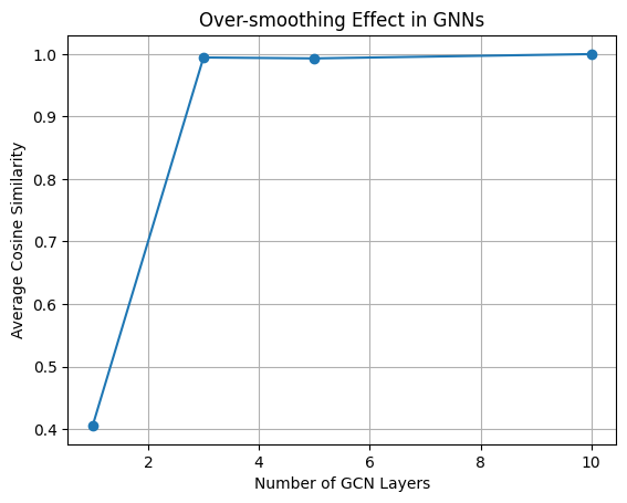
Interpretation of Results
| Depth | Similarity | What It Means | Practical Impact |
|---|---|---|---|
| 1 layer | 0.406 | Nodes still distinct | Can identify different atoms |
| 3 layers | 0.995 | Nearly identical | Losing atomic identity |
| 5 layers | 0.993 | Effectively same | No useful information |
| 10 layers | 1.000 | Complete collapse | Model is useless |
As shown above, as the number of message-passing layers increases, node representations converge. Initially distinct feature vectors (left) become nearly indistinguishable after several layers (right), resulting in the loss of structural information. This phenomenon is known as over-smoothing and is a critical limitation of deep GNNs.
Interpretation
As we can see, even at just 3 layers, the node embeddings become nearly identical. By 10 layers, the model has effectively lost all ability to distinguish individual atoms. This is the core issue of over-smoothing—deep GNNs can blur out meaningful structural differences.
Solutions to Over-smoothing
| Technique | How It Works | Implementation | Effectiveness |
|---|---|---|---|
| Residual Connections | Skip connections preserve original features | x = x + GCN(x) | Very effective |
| Feature Concatenation | Combine features from multiple layers | concat(x₁, x₂, ...) | Good for shallow nets |
| Batch Normalization | Normalize features per layer | BatchNorm after GCN | Moderate help |
| Jumping Knowledge | Aggregate all layer outputs | JK networks | State-of-the-art |
To mitigate this problem, modern GNNs use techniques like:
- Residual connections (skip connections that reintroduce raw input)
- Feature concatenation from earlier layers
- Batch normalization or graph normalization
- Jumping knowledge networks to combine representations from multiple layers
When working with molecular graphs, you should choose the depth of your GNN carefully. It should be deep enough to capture important substructures, but not so deep that you lose atomic-level details.
Interpretability in Molecular GNNs
Beyond the technical challenge of over-smoothing, GNNs face a critical issue of interpretability. When a model predicts that a molecule might be toxic or have specific properties, chemists need to understand which structural features drive that prediction. This “black box” nature of neural networks is particularly problematic in chemistry, where understanding structure-activity relationships is fundamental to rational drug design.
Why Interpretability Matters in Chemistry
| Stakeholder | Need | Example | Impact |
|---|---|---|---|
| Medicinal Chemists | Understand SAR Structure-Activity Relationships |
Which groups increase potency? | Guide drug optimization |
| Regulatory Bodies | Safety justification Why is it safe? |
Explain toxicity predictions | FDA approval |
| Researchers | Scientific insight New mechanisms |
Discover new pharmacophores | Advance knowledge |
| Industry | Risk assessment Confidence in predictions |
Why invest in this molecule? | Resource allocation |
Recent advances in GNN interpretability for molecular applications have taken several promising directions:
Attention-Based Methods:
| Attention-Based Interpretability | |||
|---|---|---|---|
|
Method: Graph Attention Networks GATs |
How it works: Learn importance weights α_ij for each edge |
Visualization: Highlight important bonds Thicker = more important |
Reference: Veličković et al., 2017 ICLR |
Graph Attention Networks (GATs) provide built-in interpretability through their attention mechanisms, allowing researchers to visualize which atoms or bonds the model considers most important for a given prediction [1,2]. This approach naturally aligns with chemical intuition about reactive sites and functional groups.
Substructure-Based Explanations:
| Substructure Mask Explanation (SME) | |||
|---|---|---|---|
|
Innovation: Fragment-based Not just atoms |
Alignment: Chemical intuition Functional groups |
Application: Toxicophore detection Find toxic substructures |
Reference: Nature Comms, 2023 14, 2585 |
The Substructure Mask Explanation (SME) method represents a significant advance by providing interpretations based on chemically meaningful molecular fragments rather than individual atoms or edges [3]. This approach uses established molecular segmentation methods to ensure explanations align with chemists’ understanding, making it particularly valuable for identifying pharmacophores and toxicophores.
Integration of Chemical Knowledge:
| Pharmacophore-Integrated GNNs | |||
|---|---|---|---|
|
Concept: Hierarchical modeling Multi-level structure |
Benefit 1: Better performance Domain knowledge helps |
Benefit 2: Natural interpretability Pharmacophore-level |
Reference: J Cheminformatics, 2022 14, 49 |
Recent work has shown that incorporating pharmacophore information hierarchically into GNN architectures not only improves prediction performance but also enhances interpretability by explicitly modeling chemically meaningful substructures [4]. This bridges the gap between data-driven learning and domain expertise.
Gradient-Based Attribution:
| SHAP for Molecular GNNs | |||
|---|---|---|---|
|
Method: SHapley values Game theory based |
Advantage: Rigorous foundation Additive features |
Output: Feature importance Per atom/bond |
Reference: Lundberg & Lee, 2017 NeurIPS |
Methods like SHAP (SHapley Additive exPlanations) have been successfully applied to molecular property prediction, providing feature importance scores that help identify which molecular characteristics most influence predictions [5,6]. These approaches are particularly useful for understanding global model behavior across different molecular classes.
Comparative Studies:
| GNNs vs Traditional Methods | |||
|---|---|---|---|
| Aspect | GNNs | Descriptor-based | Recommendation |
| Performance |
Often superior Complex patterns |
Good baseline Well-understood |
Task-dependent |
| Interpretability |
Challenging Requires extra work |
Built-in Known features |
Hybrid approach |
| Reference | Jiang et al., 2021, J Cheminformatics | ||
Recent comparative studies have shown that while GNNs excel at learning complex patterns, traditional descriptor-based models often provide better interpretability through established chemical features, suggesting a potential hybrid approach combining both paradigms [6].
The Future: Interpretable-by-Design
The field is moving toward interpretable-by-design architectures rather than post-hoc explanation methods. As noted by researchers, some medicinal chemists value interpretability over raw accuracy if a small sacrifice in performance can significantly enhance understanding of the model's reasoning [3]. This reflects a broader trend in molecular AI toward building systems that augment rather than replace human chemical intuition.
| Design Principle | Implementation | Example |
|---|---|---|
| Chemical hierarchy | Multi-scale architectures | Atom → Group → Molecule |
| Explicit substructures | Pharmacophore encoding | H-bond donors as nodes |
| Modular predictions | Separate property modules | Solubility + Toxicity branches |
Summary
Key Takeaways: Challenges and Solutions
| Challenge | Impact | Current Solutions | Future Directions |
|---|---|---|---|
| Over-smoothing | Limits depth to 3-5 layers Can't capture long-range |
• Residual connections • Jumping knowledge • Normalization |
Novel architectures Beyond message passing |
| Interpretability | Low trust & adoption Can't guide design |
• Attention visualization • SHAP values • Substructure masking |
Interpretable-by-design Chemical hierarchy |
The Path Forward:
- Balance accuracy with interpretability - Sometimes 90% accuracy with clear explanations beats 95% black box
- Incorporate domain knowledge - Chemical principles should guide architecture design
- Develop hybrid approaches - Combine GNN power with traditional descriptor interpretability
- Focus on augmenting chemists - Tools should enhance, not replace, human expertise
The challenges facing molecular GNNs—over-smoothing and interpretability—are significant but surmountable. Over-smoothing limits the depth of networks we can effectively use, constraining the model’s ability to capture long-range molecular interactions. Meanwhile, the interpretability challenge affects trust and adoption in real-world applications where understanding model decisions is crucial.
Current solutions include architectural innovations like residual connections to combat over-smoothing, and various interpretability methods ranging from attention visualization to substructure-based explanations. The key insight is that effective molecular AI systems must balance predictive power with chemical interpretability, ensuring that models not only make accurate predictions but also provide insights that align with and enhance human understanding of chemistry.
As the field progresses, the focus is shifting from purely accuracy-driven models to systems that provide transparent, chemically meaningful explanations for their predictions. This evolution is essential for GNNs to fulfill their promise as tools for accelerating molecular discovery and understanding.
References (3.3.4)
- Veličković, P., Cucurull, G., Casanova, A., Romero, A., Liò, P., & Bengio, Y. (2017). Graph Attention Networks. International Conference on Learning Representations.
- Yuan, H., Yu, H., Gui, S., & Ji, S. (2022). Explainability in graph neural networks: A taxonomic survey. IEEE Transactions on Pattern Analysis and Machine Intelligence.
- Chemistry-intuitive explanation of graph neural networks for molecular property prediction with substructure masking. (2023). Nature Communications, 14, 2585.
- Integrating concept of pharmacophore with graph neural networks for chemical property prediction and interpretation. (2022). Journal of Cheminformatics, 14, 52.
- Lundberg, S. M., & Lee, S. I. (2017). A unified approach to interpreting model predictions. Advances in Neural Information Processing Systems, 30, 4765-4774.
- Jiang, D., Wu, Z., Hsieh, C. Y., Chen, G., Liao, B., Wang, Z., … & Hou, T. (2021). Could graph neural networks learn better molecular representation for drug discovery? A comparison study of descriptor-based and graph-based models. Journal of Cheminformatics, 13(1), 1-23.
-
Section 3.3 – Quiz Questions
1) Factual Questions
Question 1
What is the primary advantage of using Graph Neural Networks (GNNs) over traditional neural networks for molecular property prediction?
A. GNNs require less computational resources
B. GNNs can directly process the graph structure of molecules
C. GNNs always achieve higher accuracy than other methods
D. GNNs work only with small molecules
▶ Click to show answer
Correct Answer: B▶ Click to show explanation
Explanation: GNNs can directly process molecules as graphs where atoms are nodes and bonds are edges, preserving the structural information that is crucial for determining molecular properties.Question 2
In the message passing mechanism of GNNs, what happens during the aggregation step?
A. Node features are updated using a neural network
B. Messages from neighboring nodes are combined
C. Edge features are initialized
D. The final molecular prediction is made
▶ Click to show answer
Correct Answer: B▶ Click to show explanation
Explanation: During aggregation, all incoming messages from neighboring nodes are combined (typically by summing or averaging) to form a single aggregated message for each node.Question 3
Which of the following molecular representations is most suitable as input for a Graph Neural Network?
A. SMILES string directly as text
B. 2D image of the molecular structure
C. Graph with nodes as atoms and edges as bonds
D. List of molecular descriptors only
▶ Click to show answer
Correct Answer: C▶ Click to show explanation
Explanation: GNNs are designed to work with graph-structured data where nodes represent atoms and edges represent chemical bonds, allowing the model to learn from the molecular connectivity.Question 4
What is the “over-smoothing” problem in Graph Neural Networks?
A. The model becomes too complex to train
B. Node representations become increasingly similar in deeper networks
C. The model cannot handle large molecules
D. Training takes too much time
▶ Click to show answer
Correct Answer: B▶ Click to show explanation
Explanation: Over-smoothing occurs when deep GNNs make node representations increasingly similar across layers, losing the ability to distinguish between different atoms and their local environments.2) Conceptual Questions
Question 5
You want to build a GNN to predict molecular solubility (a continuous value). Which combination of pooling and output layers would be most appropriate?
A.
# Mean pooling + regression output
x = global_mean_pool(x, batch)
output = nn.Linear(hidden_dim, 1)(x)
B.
# Max pooling + classification output
x = global_max_pool(x, batch)
output = nn.Sequential(nn.Linear(hidden_dim, 2), nn.Softmax())(x)
C.
# No pooling + multiple outputs
output = nn.Linear(hidden_dim, num_atoms)(x)
D.
# Sum pooling + sigmoid output
x = global_add_pool(x, batch)
output = nn.Sequential(nn.Linear(hidden_dim, 1), nn.Sigmoid())(x)
▶ Click to show answer
Correct Answer: A▶ Click to show explanation
Explanation: For continuous property prediction (regression), we need to pool node features to get a molecular-level representation, then use a linear layer to output a single continuous value. Mean pooling is commonly used and effective for this purpose.▶ Click to see code: Complete GNN architecture for solubility prediction
# Complete GNN for solubility prediction
class SolubilityGNN(nn.Module):
    def __init__(self, node_features, hidden_dim=64):
        super(SolubilityGNN, self).__init__()
        self.conv1 = GCNConv(node_features, hidden_dim)
        self.conv2 = GCNConv(hidden_dim, hidden_dim)
        self.predictor = nn.Linear(hidden_dim, 1)

    def forward(self, x, edge_index, batch):
        x = F.relu(self.conv1(x, edge_index))
        x = F.relu(self.conv2(x, edge_index))
        x = global_mean_pool(x, batch)  # Pool to molecular level
        return self.predictor(x)        # Single continuous output
Question 6
A chemist notices that their GNN model performs well on training molecules but poorly on a new set of structurally different compounds. What is the most likely cause and solution?
A. The model is too simple; add more layers
B. The model suffers from distribution shift; collect more diverse training data
C. The learning rate is too high; reduce it
D. The model has too many parameters; reduce model size
▶ Click to show answer
Correct Answer: B▶ Click to show explanation
Explanation: This scenario describes distribution shift, where the model was trained on one chemical space but tested on a different one. The solution is to include more diverse molecular structures in the training data to improve generalization.▶ Click to see code: Data augmentation for chemical space diversity
# Data augmentation to improve generalization
def augment_chemical_space(original_smiles_list):
    """Expand training data with structural diversity"""
    augmented_data = []

    for smiles in original_smiles_list:
        mol = Chem.MolFromSmiles(smiles)

        # Add original
        augmented_data.append(smiles)

        # Add different SMILES representations
        for _ in range(3):
            random_smiles = Chem.MolToSmiles(mol, doRandom=True)
            augmented_data.append(random_smiles)

    return augmented_data

# Use diverse training data from multiple chemical databases
diverse_training_data = combine_datasets([
    'drug_molecules.csv',
    'natural_products.csv',
    'synthetic_compounds.csv'
])