2. Preliminaries

In the Preliminaries chapter, we will introduce some base coding and data analysis.

2.1 Introduction to Python

This section covers essential Python skills, including setting up your environment, understanding basic syntax, and using packages to aid data analysis. This foundational knowledge is valuable for beginners and will support more advanced data analysis in later sections.

2.1.1 Setting up Python Environment

Option 1: Using Google Colab

Google Colab is a cloud-based platform for running Python code in what are called notebooks, which section code in to small chunks that can be run independently. Dividing a program into small sections is helpful for data science and machine learning. Follow these steps to get started. Using Google Colab allows you to run Python code in a flexible, collaborative environment without any local setup. It’s particularly useful for working with large datasets or sharing notebooks with others.

Step 1: Access Google Colab

Open Google Colab: Go to Google Colab.
Sign in with Google: Log in with your Google account to access and save notebooks in Google Drive.

Step 2: Create or Open a Notebook

Create a New Notebook:
- Click on File > New notebook to open a blank notebook.
Open an Existing Notebook:
- Choose File > Open notebook. You can load notebooks from Google Drive, GitHub, or your computer.

Step 3: Set Up and Run Code

Using Code Cells:
- Colab organizes code into cells. To run a cell, click on it and press Shift + Enter or click the Play button.
Installing Packages
Colab has many libraries installed by default. You can install additional packages if needed using pip commands within a cell.

# Install additional libraries
!pip install some_package

Library	Purpose	Pip Install Command
`rdkit`	Cheminformatics tasks: SMILES, molecular fingerprints, 3D coordinates, etc.	`pip install rdkit-pypi`
`pandas`	Data manipulation and analysis.	`pip install pandas`
`numpy`	Numerical computing support.	`pip install numpy`
`matplotlib`	Data visualization (histograms, plots, etc.).	`pip install matplotlib`
`seaborn`	Advanced statistical plotting.	`pip install seaborn`
`scikit-learn`	Machine learning: regression, clustering, model evaluation.	`pip install scikit-learn`
`scipy`	Scientific computing: statistical tests (e.g., `f_oneway`), optimization, etc.	`pip install scipy`
`plotly`	Interactive plots and dashboards.	`pip install plotly`

Step 4: Save and Export Your Work

Saving to Google Drive:
- Your Colab notebooks will automatically save to Google Drive. You can access them later under Colab Notebooks in Drive.
Downloading Notebooks:
- To keep a copy on your computer, go to File > Download > Download .ipynb.

Step 5: Loading Files and Datasets in Colab

Mount Google Drive:
- Run the following code to access your files on Google Drive. After running, authorize access to your Drive.
```
from google.colab import drive
drive.mount('/content/drive')
```
Load Local Files:
- Use Colab’s file upload feature by clicking the File icon on the left sidebar, then selecting Upload Notebook.

Step 6: Adding and Executing Markdown Cells

Adding Markdown for Documentation:
- To add notes, explanations, or instructions in text, you can insert a Markdown cell by clicking + Text in the toolbar.

Tips for Chemists Using Colab

Managing Data Files: Store datasets in Google Drive to access them easily across multiple sessions.
Running Long Calculations: Colab may disconnect if idle. To prevent data loss, make sure to save work frequently.
Collaborative Editing: Share Colab notebooks with colleagues for real-time collaboration by clicking Share in the top-right corner.

Option 2: Installing Anaconda and Jupyter Notebook

To get started with Python, we’ll set up a development environment using Anaconda and Jupyter Notebook.

Anaconda: A package manager and environment manager commonly used for data science. It simplifies package installation and management.
Jupyter Notebook: An interactive environment ideal for data exploration and analysis. Jupyter Notebooks can be launched directly from Anaconda.

Here’s a detailed guide on installing Anaconda on different operating systems. Each step is tailored for Windows, macOS, and Linux to ensure a smooth setup.

Installing Anaconda on Windows, macOS, and Linux

Download Anaconda

Go to the Anaconda Download Page:
- Visit the Anaconda download page.
Select Your Operating System:
- Choose the appropriate installer for your OS: Windows, macOS, or Linux.
- Select the Python 3.x version (e.g., Python 3.9 or 3.10) for the latest stable release.
- Anaconda may detect your operating system and only give one option to download.

Windows Installation Instructions

Run the Installer:
- Open the downloaded .exe file.
- Click Next on the Welcome screen.
Agree to the License Agreement:
- Read the agreement, then click I Agree.
Select Installation Type:
- Choose Just Me unless multiple users need access.
Choose Installation Location:
- Choose the default or specify a custom path.
- Avoid spaces or special characters in the path if choosing a custom location.
Advanced Installation Options:
- Check Add Anaconda to my PATH environment variable (optional but not recommended due to potential conflicts).
- Ensure Register Anaconda as my default Python 3.x is selected, so Anaconda’s Python is used by default.
Complete the Installation:
- Click Install and wait for the process to finish.
- Once complete, you can choose to open Anaconda Navigator or continue with manual setup.
Verify the Installation:
- Open Anaconda Prompt from the Start Menu.
- Type conda --version to verify the installation.
- Launch Jupyter Notebook by typing jupyter notebook.

macOS Installation Instructions

Run the Installer:
- Open the downloaded .pkg file.
- Follow the prompts on the installer.
Agree to the License Agreement:
- Review and agree to the terms to proceed.
Choose Installation Location:
- By default, Anaconda is installed in the /Users/username/anaconda3 directory.
Advanced Options:
- You may be asked if you want Anaconda’s Python to be your default Python.
- Choose Yes to add Anaconda to your PATH automatically.
Complete the Installation:
- Wait for the installation to complete, then close the installer.
Verify the Installation:
- Open Terminal.
- Type conda --version to verify that Anaconda is installed.
- Launch Jupyter Notebook by typing jupyter notebook.

Linux Installation Instructions

Open Terminal.
Navigate to the Download Directory:
- Use cd to navigate to where you downloaded the Anaconda installer.
```
cd ~/Downloads
```
Run the Installer:
- Run the installer script. Replace Anaconda3-202X.X.X-Linux-x86_64.sh with your specific file name.
```
bash Anaconda3-202X.X.X-Linux-x86_64.sh
```
Review the License Agreement:
- Press Enter to scroll through the agreement.
- Type yes when prompted to accept the agreement.
Specify Installation Location:
- Press Enter to accept the default installation path (/home/username/anaconda3), or specify a custom path.
Add Anaconda to PATH:
- Type yes when asked if the installer should initialize Anaconda3 by running conda init.
Complete the Installation:
- Once installation is finished, restart the terminal or use source ~/.bashrc to activate the changes.
Verify the Installation:
- Type conda --version to confirm that Anaconda is installed.
- Launch Jupyter Notebook by typing jupyter notebook.

Post-Installation: Launch Jupyter Notebook

Open Anaconda Prompt (Windows) or Terminal (macOS/Linux).
Start Jupyter Notebook:
- Type jupyter notebook and press Enter.
- Jupyter Notebook will open in your default web browser, allowing you to create and run Python code interactively.

2.1.2 Basic Syntax and Structure

Python’s simple syntax makes it a powerful and beginner-friendly language for data analysis. Here, we’ll cover core aspects:

Variables, Loops, and Functions

Variables: Used to store data. You can define a variable by simply assigning it a value.

# Defining variables
compound_name = "Aspirin"
molecular_weight = 180.16

Loops: Used to perform repetitive tasks.

# For loop example
for i in range(3):
   print(f"Compound {i+1}")

Functions: Functions in Python allow you to reuse blocks of code and organize your script.

# Function to calculate the molecular weight ratio
def molecular_weight_ratio(compound_weight, standard_weight=100):
   return compound_weight / standard_weight

print(molecular_weight_ratio(molecular_weight))

Data Types and Mathematical Operations

Data Types: How data such as a variable is represented to and stored in the computer.

string type: Data meant to be interpreted literally
integer type: Data meant to be stored as an integer
float type: Data meant to be stored as a floating point number with decimal precision

Example Code

# Display the data type of variables
my_string = "10"
my_int = 10
my_float = 10.0

print(type(my_string))
print(type(my_int))
print(type(my_float))

Output

<class 'str'>
<class 'int'>
<class 'float'>

Mathematical Operations: The four regular mathematical operations can be used on integer and float type variables and order of operations is followed.

Addition with the “+” character
Substraction with the “-“ character
Multiplication with the “*” character
Division with the “/” character

Example Code

# Use the mathematical operators
my_int = 10

print(my_int * 3 / 2 + 1 - 3)

Output

13.0

Basic Printing Techniques in Python

Print commands are used in most programming languages to display the output of code that has been run. Printing is essential for checking code functionality, displaying calculations, and formatting data. Here are a few common ways to print in Python, along with examples that can help navigate real-world coding scenarios.

Simple Print Statements

Explanation: The print() function displays text or values to the screen. You can print variables or text strings directly.

Example Code

# Basic print
print("Welcome to Python programming!")

# Printing a variable
compound_name = "Aspirin"
print("Compound:", compound_name)

Output

Welcome to Python programming!
Compound: Aspirin

Using f-strings for Formatted Output

Explanation: Python’s formatted strings known as f-strings make it easy to display the value of a variable along with or embedded in other text, which simplifies displaying complex data clearly.

Example Code

compound_name = "Aspirin"
molecular_weight = 180.16
print(f"The molecular weight of {compound_name} is {molecular_weight}")

Output

The molecular weight of Aspirin is 180.16

Concatenating Strings and Variables

Explanation: Concatenating, or combining strings and variables is possible using the + operator, but the variable must first be converted to a string.

Example Code

print("The molecular weight of " + compound_name + " is " + str(molecular_weight))

Output

The molecular weight of Aspirin is 180.16

Formatting Numbers

Explanation: To control the display of floating-point numbers (e.g., limiting decimal places), use formatting options within f-strings.

Example Code

molecular_weight = 180.16
# Display molecular weight with two decimal places
print(f"Molecular weight: {molecular_weight:.2f}")

Output

Molecular weight: 180.16

Practice Problem

Write a program to define variables for the name and molecular weight of the active compound in Ibuprofen. Display the information using each print method above.

▶ Show Solution Code


compound_name = "Ibuprofen"
molecular_weight = 206.29

# Simple print
print("Compound:", compound_name)

# f-string
print(f"The molecular weight of {compound_name} is {molecular_weight}")

# Concatenation
print("The molecular weight of " + compound_name + " is " + str(molecular_weight))

# Formatting numbers
print(f"Molecular weight: {molecular_weight:.2f}")

2.1.3 Python Packages

Python packages are pre-built libraries that simplify data analysis. Here, we’ll focus on a few essential packages for our work.

Key Packages

NumPy: A popular package for numerical computing, especially helpful for handling arrays and performing mathematical operations.
Pandas: A popular library for data manipulation, ideal for handling tabular data structures like the contents of a spreadsheet.
Matplotlib and Seaborn: Libraries for data visualization in plots and figures.

Example Code to Install and Import Packages

# Installing packages
!pip install numpy pandas matplotlib seaborn

# Importing packages
import numpy as np
import pandas as pd
import matplotlib.pyplot as plt
import seaborn as sns

To load data from any file into your program, the program needs to know where to find the file. This can be accomplished in one of two ways. In the following example, we will load a text file.

Place the file inside the same folder as your program and open the file by its name:

# Loading data from a text file in the same location as your program
with open('data.txt') as f:
   data = f.read()

Find the full directory path to your file and provide this as the file name. In Windows, you can right click a file in File Explorer and click on “Copy as path” to copy the full directory path to your file. For example, if user coolchemist has the file ‘data.txt’ in their Desktop folder, the code to load this file might look like this:
```
# Loading data from a text file in the Desktop folder of user coolchemist
with open('C:\Users\coolchemist\Desktop\data.txt') as f:
   data = f.read()
```

Practice Problem:

Problem: Write Python code to create a variable for a compound’s molecular weight and set it to 180.16. Then create a function that doubles the molecular weight.

▶ Show Solution Code


# Define a variable for molecular weight
molecular_weight = 180.16

# Function to double the molecular weight
def double_weight(weight):
   return weight * 2

# Test the function
print(f"Double molecular weight: {double_weight(molecular_weight)}")

Output

Double molecular weight: 360.32

2.2 Data Analysis with Python

In this chapter, we’ll explore how to use Python for data analysis, focusing on importing and managing datasets commonly encountered in chemistry. Data analysis is a crucial skill for chemists, allowing you to extract meaningful insights from experimental data, predict outcomes, and make informed decisions in your research. Effective data analysis begins with properly importing and managing your datasets. This section will guide you through loading data from various file formats, including those specific to chemistry, and handling data from databases.

2.2.1 Loading Data from Various File Formats

Completed and Compiled Code: Click Here

Reading Data from CSV

Explanation:

CSV (Comma-Separated Values) and Excel files are common formats for storing tabular data. Python’s pandas library provides straightforward methods to read these files into DataFrames, which are powerful data structures for working with tabular data. A DataFrame is what is known in programming as an object. Objects contain data organized in specific defined structures and have properties that can be changed and used by the programmer.

Think of it as a variable that can store more complex information than a few words or a number. In this instance, we will store data tables as a DataFrame object. When the data table is read into a pandas DataFrame, the resulting object will have properties and functions built into it. For example, a substrate scope table can be read into a DataFrame and statistical analysis can be performed on the yield column with only a few lines of code.

Example Code:

import pandas as pd

# Reading a CSV file into a DataFrame called "csv_data"
csv_data = pd.read_csv('experimental_data.csv')

# Reading an Excel file into a DataFrame called "excel_data"
excel_data = pd.read_excel('compound_properties.xlsx', sheet_name='Sheet1', index_col=0)

Explanation of the Code:

pd.read_csv() reads data from a CSV file into a DataFrame.
pd.read_excel() reads data from an Excel file. The sheet_name parameter specifies which sheet to read. The index_col parameter tells pandas which column to use as the row index.

Note: What is index_col?

When loading an Excel file with pandas.read_excel(), pandas automatically assigns row numbers like 0, 1, 2 as the index. But sometimes, the first column of your file already contains meaningful labels—like wavenumbers, timestamps, or compound IDs. In that case, you can tell pandas to use that column as the row index using index_col.

Without index_col

Suppose your Excel file starts with a column named “Wavenumber”, followed by data columns like “Time1” and “Time2”. If you don’t set index_col, pandas reads all columns as data. It then adds its own row numbers—0, 1, 2—on the side. The “Wavenumber” column will just be treated as another data column.

With index_col=0

By setting index_col=0, you’re telling pandas to treat the first column—“Wavenumber”—as the index. That means each row will now be labeled using the values in the “Wavenumber” column (e.g., 400, 500, 600). This is especially useful when the first column isn’t a feature but a meaningful label.

Reading CSVs via File Upload or Link

You can read CSV files in two ways:

Method 1: Upload the file manually (e.g., in Jupyter or Google Colab)

Download the BBBP.csv File: Click Here

from google.colab import files
uploaded = files.upload()
   
import pandas as pd
df = pd.read_csv('BBBP.csv')
# .head() gets the first 5 rows
print(df.head())

Method 2: Load the file directly from a GitHub raw link

This method allows your code to be instantly runnable without needing to manually upload files.

import pandas as pd

# Loading the dataset
url = 'https://raw.githubusercontent.com/Data-Chemist-Handbook/Data-Chemist-Handbook.github.io/refs/heads/master/_pages/BBBP.csv'
df = pd.read_csv(url)
print(df.head())

Output

   num                  name  p_np                                             smiles
  1            Propanolol     1                   [Cl].CC(C)NCC(O)COc1cccc2ccccc12
  2  Terbutylchlorambucil     1           C(=O)(OC(C)(C)C)CCCc1ccc(cc1)N(CCCl)CCCl
  3                 40730     1  c12c3c(N4CCN(C)CC4)c(F)cc1c(c(C(O)=O)cn2C(C)CO...
  4                    24     1                   C1CCN(CC1)Cc1cccc(c1)OCCCNC(=O)C
  5           cloxacillin     1  Cc1onc(c2ccccc2Cl)c1C(=O)N[C@H]3[C@H]4SC(C)(C)...

Note: Method 2 works for CSVs but not for Excel files

CSV files are plain text files. When you use a raw.githubusercontent.com link, you’re simply accessing that text over the internet, and pandas.read_csv() can parse it just like it would read from a local file.

Excel files (.xlsx), however, are binary files, not plain text. GitHub doesn’t serve .xlsx files with the correct content type to let pd.read_excel() work directly from the URL. Instead, you need to manually download the file into memory using the requests library and wrap it with BytesIO, like this:

import pandas as pd
import requests
from io import BytesIO

url = 'https://raw.githubusercontent.com/Data-Chemist-Handbook/Data-Chemist-Handbook.github.io/master/_pages/LCRaman_data.xlsx'
response = requests.get(url)
excel_data = BytesIO(response.content)

df = pd.read_excel(excel_data, sheet_name='Sheet1', index_col=0)
print(df.head())

Output

                  time       4.5  4.533333 ... 7.433333  7.466667
40mM amino acids                                                                                                                                                                                               
wavenumber/cm-1    NaN       NaN       NaN ...      NaN       NaN
325.65             NaN  0.003956  0.003982 ... 0.012759  0.014740
327.651677         NaN  0.005396  0.004230 ... 0.012213  0.014480
329.652707         NaN  0.004024  0.005562 ... 0.012120  0.012711
331.65309          NaN  0.003313  0.005206 ... 0.009913  0.011362

[5 rows x 91 columns]

2.2.2 Data Cleaning and Preprocessing

Completed and Compiled Code: Click Here

Handling Missing Values and Duplicates

Because datasets often combine data from multiple sources or are taken from large databases, they need to be processed before being analyzed to prevent using incomplete or incorrect data. The processing is called cleaning and can be done with the help of built in functions rather than through manual fixing.

Explanation: Data cleaning can be done with built in functions of the DataFrame object. This example uses fillna() to fill missing values with specified values and drop_duplicates() to remove duplicate rows from the DataFrame.

Example Code:

import pandas as pd

# Create a sample dataset with some missing 'name' values and duplicate 'smiles'
data = {
    'name': ['Aspirin', None, 'Ibuprofen', 'Aspirin', None],
    'smiles': ['CC(=O)OC1=CC=CC=C1C(=O)O', 'CC(=O)OC1=CC=CC=C1C(=O)O', 'CC(C)CC1=CC=C(C=C1)C(C)C(=O)O', '', '']
}
df = pd.DataFrame(data)

# Number of rows before removing duplicates
initial_row_count = len(df)

# Count how many rows have missing values in the 'name' column using isna() (checks for NaN) and sum() (counts total)
missing_name_count = df['name'].isna().sum()

# Handle missing values
df_filled = df.fillna({'name': 'Unknown', 'smiles': ''})

# Remove duplicate rows based on the 'smiles' column; 'subset' specifies which column(s) to consider for identifying duplicates
df_no_duplicates = df_filled.drop_duplicates(subset=['smiles'])

# Final row count after removing duplicates
final_row_count = len(df_no_duplicates)

# Print results
print(f"Number of rows before removing duplicates: {initial_row_count}")
print(f"Number of rows with missing names (filled as 'Unknown'): {missing_name_count}")
print(f"Number of rows after removing duplicates: {final_row_count}")

Output

Number of rows before removing duplicates: 5
Number of rows with missing names (filled as 'Unknown'): 2
Number of rows after removing duplicates: 3

Practice Problem:

We will clean the dataset by filling missing name values with 'Unknown', removing rows without smiles values, and removing any duplicate entries based on smiles.

Given a DataFrame with missing values:

Fill missing values in the name column with 'Unknown' and in the smiles column with an empty string.
Remove any duplicate rows based on the smiles column.

▶ Click to show considerations

In this practice problem, we removed data rows that did not contain `smiles` info, but what if we wanted to attempt to fill in the data based on the name? There are ways to do this through other python packages, such as pubchempy.

Data Type Conversions

Explanation: Converting data types to the desired type for a given data category enables proper representation of the data for performing mathematical calculations or comparisons. This is necessary when data is imported with incorrect types (e.g., numbers stored as strings).

Example Code:

import pandas as pd

# Example DataFrame with mixed types
data = {'product': [1, 2, 3],
      'milligrams': ['10.31', '8.04', '3.19'],
      'yield': ['75', '46', '32']}
df = pd.DataFrame(data)

print("the data types before conversion are:")
print(str(df.dtypes) + "\n")

# Converting 'product' to string
df['product'] = df['product'].astype(str)

# Converting 'milligrams' to float
df['milligrams'] = df['milligrams'].astype(float)

# Converting 'yield' to integer
df['yield'] = df['yield'].astype(int)

print("the data types after conversion are:")
print(str(df.dtypes))

Output

the data types before conversion are:
product        int64
milligrams    object
yield         object
dtype: object

the data types after conversion are:
product        object
milligrams    float64
yield           int64
dtype: object

Note: In pandas, dtype: object means the column can hold any Python object, most commonly strings. Practice Problem: In the BBBP dataset, the num column (compound number) should be treated as an integer, and the p_np column (permeability label) should be converted to categorical data.

Convert the num column to integer and the p_np column to a categorical type.
Verify that the conversions are successful by printing the data types.

▶ Show Solution Code


import pandas as pd

# Loading the dataset again
url = 'https://raw.githubusercontent.com/Data-Chemist-Handbook/Data-Chemist-Handbook.github.io/refs/heads/master/_pages/BBBP.csv'
df = pd.read_csv(url)

# Convert 'num' to integer and 'p_np' to categorical
df['num'] = df['num'].astype(int)
df['p_np'] = df['p_np'].astype('category')

# Print the data types of the columns
print(df.dtypes)

Output

num          int64
name        object
p_np      category
smiles      object
dtype: object

Normalizing and Scaling Data

Because different features may span very different ranges, it’s often useful to bring them onto a common scale before modeling.

Explanation: Normalization adjusts the values of numerical columns to a common scale without distorting differences in ranges. This is often used in machine learning algorithms to improve model performance by making data more comparable.

Note: In cheminformatics, the term normalization can also refer to structural standardization (e.g., canonicalizing SMILES to avoid duplicates), as discussed in Walters et al., Nature Chemistry (2021). However, in machine learning, normalization usually refers to mathematical feature scaling (e.g., Min–Max or z-score scaling).

Note: Since different features may span very different ranges, it’s often useful to bring them onto a common scale before modeling. Machine learning models expect

Rows = individual samples or observations (e.g., a single spectrum)
Columns = features (e.g., intensity at different wavenumbers) If your data is organized the other way around (e.g., rows as wavenumbers), use .T to transpose the DataFrame: df = df.T.

Note: Not every chemical column should be re-scaled.
Physical constants such as boiling-point (°C/K), pH, melting-point, ΔHf, etc. already live on a meaningful, absolute scale; forcing them into 0-1 space can hide or even distort mechanistic trends.

By contrast, measurement-derived signals (e.g. FTIR, Raman or UV-Vis intensities) and vectorised descriptors produced by software (atom counts, fragment fingerprints, Mordred/PaDEL descriptors, etc.) are scalable. Re-scaling these routinely improves machine-learning performance and does not alter the underlying chemistry.

Example Code:

import pandas as pd
from sklearn.preprocessing import MinMaxScaler

# Toy IR-intensity dataset (three peaks per spectrum)
spectra = pd.DataFrame({
    "sample": ["spec-1", "spec-2", "spec-3"],
    "I_1700cm-1": [  920,  415, 1280],
    "I_1600cm-1": [  640, 1220,  870],
    "I_1500cm-1": [  305,  510,  460],
})

scaler = MinMaxScaler()
intensity_cols = ["I_1700cm-1", "I_1600cm-1", "I_1500cm-1"]

spectra[intensity_cols] = scaler.fit_transform(spectra[intensity_cols])
print(spectra)

Output: | | sample | I_1700cm-1 | I_1600cm-1 | I_1500cm-1 | |——–|———|————|————|————| | 0 | spec-1 | 0.583815 | 0.000000 | 0.000000 | | 1 | spec-2 | 0.000000 | 1.000000 | 1.000000 | | 2 | spec-3 | 1.000000 | 0.396552 | 0.756098 |

Practice Problem:

We will normalize Raman spectral intensity data using Min–Max scaling, which adjusts values to a common scale between 0 and 1.

Load LCRaman_data.xlsx from the GitHub repository. This file contains real Raman spectral measurements.
Transpose the DataFrame to make rows = spectra and columns = wavenumber intensities.
Apply Min–Max scaling to the intensity values.
Print the first few rows to verify the normalized values.

▶ Show Solution Code


import pandas as pd
from sklearn.preprocessing import MinMaxScaler
import requests
from io import BytesIO

# Load Raman spectral data from GitHub
url = 'https://raw.githubusercontent.com/Data-Chemist-Handbook/Data-Chemist-Handbook.github.io/master/_pages/LCRaman_data.xlsx'
response = requests.get(url)
excel_data = BytesIO(response.content)
df = pd.read_excel(excel_data, sheet_name="Sheet1", index_col=0)

# Transpose to make rows = spectra, columns = features
spectra = df.T

# Remove any rows (now columns) that aren't numeric (force numeric, NaN if not)
spectra = spectra.apply(pd.to_numeric, errors='coerce')

# Drop columns that are all NaNs (e.g. invalid features)
spectra = spectra.dropna(axis=1, how='all')

# Ensure all column names are strings to avoid errors in scikit-learn, which requires uniform string-type feature names
new_columns = []
for col in spectra.columns:
    new_columns.append(str(col))
spectra.columns = new_columns

# Apply Min–Max scaling to all intensity columns
scaler = MinMaxScaler()
spectra_scaled = pd.DataFrame(
    scaler.fit_transform(spectra),
    index=spectra.index,
    columns=spectra.columns
)

print(spectra_scaled.head())

Output

            325.65  327.65167664  ... 2033.94965376  2035.29038256
time           NaN           NaN  ...           NaN            NaN
4.5       0.751313      0.778351  ...      0.821384       0.763345
4.533333  0.751916      0.749897  ...      0.783924       0.634459
4.566667  0.810788      0.814801  ...      0.789397       0.666986
4.6       0.758148      0.819177  ...      0.756293       0.574035

Explanation of the Code: The script starts by loading Raman spectral data from an Excel file hosted on GitHub. It reads the first sheet into a pandas DataFrame, using the first column as the index. At this point, rows represent Raman shifts (wavenumbers), and columns represent sample measurements at various time points or conditions.

To prepare the data for machine learning, the DataFrame is transposed so that each row represents a spectrum (sample), and each column corresponds to a wavenumber feature. This is the standard format expected by most machine learning models: rows as observations, columns as features.

The script then converts all values to numeric using pd.to_numeric(). This step handles any non-numeric entries (e.g., text or metadata), converting them to NaN, which ensures that only valid numerical data is kept for further processing.

Next, columns that contain only NaN values are dropped. These typically result from unmeasured or corrupted wavenumbers and offer no useful information, so removing them helps clean the dataset and reduce dimensionality.

Before scaling, the script ensures all column names are strings. This is important because scikit-learn requires feature names to be of a consistent type. If a mix of float and string column names is present (common when wavenumbers are numeric), it raises a TypeError. Converting all names to strings ensures compatibility.

Finally, Min–Max scaling is applied to normalize all feature values between 0 and 1. This ensures that each wavenumber contributes equally to analyses, preventing features with large values from dominating. The first few rows of the scaled data are printed to verify the transformation.

2.2.3 Data Manipulation with Pandas

Completed and Compiled Code: Click Here

Filtering and Selecting Data

Explanation:

Filtering allows you to select specific rows or columns from a DataFrame that meet a certain condition. This is useful for narrowing down data to relevant sections.

Example Code:

import pandas as pd

# Example DataFrame
data = {'Compound': ['A', 'B', 'C'],
         'MolecularWeight': [180.16, 250.23, 320.45]}
df = pd.DataFrame(data)

# Filtering rows where MolecularWeight is greater than 200
filtered_df = df[df['MolecularWeight'] > 200]

print(filtered_df)

Output

  Compound  MolecularWeight
1        B           250.23
2        C           320.45

Practice Problem 1:

Filter a DataFrame from the BBBP dataset to show only rows where the num (compound number) is greater than 500.
Select a subset of columns from the dataset and display only the name and smiles columns.

▶ Show Solution Code


import pandas as pd

# Loading the BBBP dataset
url = 'https://raw.githubusercontent.com/Data-Chemist-Handbook/Data-Chemist-Handbook.github.io/refs/heads/master/_pages/BBBP.csv'
df = pd.read_csv(url)

# Filtering rows where the 'num' column is greater than 500
filtered_df = df[df['num'] > 500]

# Selecting a subset of columns: 'name' and 'smiles'
subset_df = df[['name', 'smiles']]

print(filtered_df.head())
print() # New line
print(subset_df.head())

Output

     num          name  p_np                                       smiles
501      buramate     1                          OCCOC(=O)NCc1ccccc1
502  butabarbital     1                 CCC(C)C1(CC)C(=O)NC(=O)NC1=O
503      caffeine     1                 Cn1cnc2N(C)C(=O)N(C)C(=O)c12
504   cannabidiol     1  CCCCCc1cc(O)c(C2C=C(C)CC[C@H]2C(C)=C)c(O)c1
505      capuride     1                      CCC(C)C(CC)C(=O)NC(N)=O

                   name                                             smiles
          Propanolol                   [Cl].CC(C)NCC(O)COc1cccc2ccccc12
Terbutylchlorambucil           C(=O)(OC(C)(C)C)CCCc1ccc(cc1)N(CCCl)CCCl
               40730  c12c3c(N4CCN(C)CC4)c(F)cc1c(c(C(O)=O)cn2C(C)CO...
                  24                   C1CCN(CC1)Cc1cccc(c1)OCCCNC(=O)C
         cloxacillin  Cc1onc(c2ccccc2Cl)c1C(=O)N[C@H]3[C@H]4SC(C)(C)...

Merging and Joining Datasets

Explanation:

Merging allows for combining data from multiple DataFrames based on a common column or index. This is especially useful for enriching datasets with additional information.

Example Code:

import pandas as pd

# Example DataFrames
df1 = pd.DataFrame({'Compound': ['A', 'B'],
                     'MolecularWeight': [180.16, 250.23]})

df2 = pd.DataFrame({'Compound': ['A', 'B'],
                     'MeltingPoint': [120, 150]})

# Merging DataFrames on the 'Compound' column
merged_df = pd.merge(df1, df2, on='Compound')

print(merged_df)

Output

  Compound  MolecularWeight  MeltingPoint
0        A           180.16           120
1        B           250.23           150

Practice Problem 2:

Merge two DataFrames from the BBBP dataset: One containing the name and smiles columns and another containing the num and p_np columns.
Perform a left join on the name column and display the result.

▶ Show Solution Code


import pandas as pd

# Loading the BBBP dataset
url = 'https://raw.githubusercontent.com/Data-Chemist-Handbook/Data-Chemist-Handbook.github.io/refs/heads/master/_pages/BBBP.csv'
df = pd.read_csv(url)

# Create two DataFrames
df1 = df[['name', 'smiles']]
df2 = df[['name', 'num', 'p_np']]

# Perform a left join on the 'name' column
merged_df = pd.merge(df1, df2, on='name', how='left')

# Print the merged DataFrame
print(merged_df.head())

Output

                   name                                             smiles  num  p_np
          Propanolol                   [Cl].CC(C)NCC(O)COc1cccc2ccccc12    1     1
Terbutylchlorambucil           C(=O)(OC(C)(C)C)CCCc1ccc(cc1)N(CCCl)CCCl    2     1
               40730  c12c3c(N4CCN(C)CC4)c(F)cc1c(c(C(O)=O)cn2C(C)CO...    3     1
                  24                   C1CCN(CC1)Cc1cccc(c1)OCCCNC(=O)C    4     1
                  24                   C1CCN(CC1)Cc1cccc(c1)OCCCNC(=O)C  667     1

Grouping and Aggregation

Explanation:

Grouping organizes data based on specific columns, and aggregation provides summary statistics like the sum, mean, or count. This is useful for analyzing data at a higher level.

Example Code:

import pandas as pd

# Example DataFrame
data = {'Compound': ['A', 'A', 'B', 'B'],
         'Measurement': [1, 2, 3, 4]}
df = pd.DataFrame(data)

# Grouping by 'Compound' and calculating the sum
grouped_df = df.groupby('Compound').sum()

print(grouped_df)

Output

          Measurement
Compound             
A                   3
B                   7

Practice Problem:

Group the BBBP dataset by p_np and compute the average carbon count for each group (permeable and non-permeable compounds).
Use multiple aggregation functions (e.g., count and mean) on the carbon count column.

▶ Show Solution Code


import pandas as pd

# Load dataset
url = 'https://raw.githubusercontent.com/Data-Chemist-Handbook/Data-Chemist-Handbook.github.io/refs/heads/master/_pages/BBBP.csv'
df = pd.read_csv(url)

# Add estimated carbon count from SMILES
df['carbon_count'] = df['smiles'].apply(lambda s: s.count('C'))

# Group by 'p_np' and calculate average carbon count
grouped_df = df.groupby('p_np')['carbon_count'].mean()

# Apply multiple aggregation functions
aggregated_df = df.groupby('p_np')['carbon_count'].agg(['count', 'mean'])

print(grouped_df)
print()
print(aggregated_df)

Output

p_np
0    14.283644
1    14.998724
Name: carbon_count, dtype: float64

      count       mean
p_np                  
0       483  14.283644
1      1567  14.998724

Pivot Tables and Reshaping Data

Explanation:

Pivot tables help reorganize data to make it easier to analyze by converting rows into columns or vice versa. This is useful for summarizing large datasets into more meaningful information.

Example Code:

import pandas as pd

# Example DataFrame
data = {'Compound': ['A', 'B', 'A', 'B'],
         'Property': ['MeltingPoint', 'MeltingPoint', 'BoilingPoint', 'BoilingPoint'],
         'Value': [120, 150, 300, 350]}
df = pd.DataFrame(data)

# Creating a pivot table
pivot_df = df.pivot_table(values='Value', index='Compound', columns='Property')

print(pivot_df)

Output

Property  BoilingPoint  MeltingPoint
Compound                            
A                300.0         120.0
B                350.0         150.0

Practice Problem 3:

Create a pivot table from the BBBP dataset to summarize the average carbon count for each p_np group (permeable and non-permeable).
Use the melt() function to reshape the DataFrame, converting columns back into rows.

▶ Show Solution Code


import pandas as pd

# Load the BBBP dataset
url = 'https://raw.githubusercontent.com/Data-Chemist-Handbook/Data-Chemist-Handbook.github.io/refs/heads/master/_pages/BBBP.csv'
df = pd.read_csv(url)

# Add carbon count derived from SMILES
df['carbon_count'] = df['smiles'].apply(lambda s: s.count('C'))

# Creating a pivot table for 'carbon_count' grouped by 'p_np'
pivot_df = df.pivot_table(values='carbon_count', index='p_np', aggfunc='mean')

# Reshaping the DataFrame using melt
melted_df = df.melt(id_vars=['name'], value_vars=['carbon_count', 'p_np'])

print(pivot_df)
print(melted_df.head())

Output

      carbon_count
p_np              
      14.283644
      14.998724
                   name      variable  value
          Propanolol  carbon_count      7
Terbutylchlorambucil  carbon_count     14
               40730  carbon_count      9
                  24  carbon_count     11
         cloxacillin  carbon_count     11

2.2.4 Working with NumPy Arrays

Completed and Compiled Code: Click Here

Basic Operations and Mathematical Functions

Explanation:

NumPy is a library for numerical computing in Python, allowing for efficient array operations, including mathematical functions like summing or averaging.

Example Code:

import numpy as np

# Example array
arr = np.array([1, 2, 3, 4, 5])

# Basic operations
arr_sum = np.sum(arr)
arr_mean = np.mean(arr)

print(f"Sum: {arr_sum}, Mean: {arr_mean}")

Output

Sum: 15, Mean: 3.0

Practice Problem 1:

Create a NumPy array from the num column in the BBBP dataset.
Perform basic statistical operations like sum, mean, and median on the num array.

▶ Show Solution Code


import pandas as pd
import numpy as np

# Load the BBBP dataset
url = 'https://raw.githubusercontent.com/Data-Chemist-Handbook/Data-Chemist-Handbook.github.io/refs/heads/master/_pages/BBBP.csv'
df = pd.read_csv(url)

# Create a NumPy array from the 'num' column
num_array = np.array(df['num'])

# Perform basic statistical operations
num_sum = np.sum(num_array)
num_mean = np.mean(num_array)
num_median = np.median(num_array)

print(f"Sum: {num_sum}, Mean: {num_mean}, Median: {num_median}")

Output

Sum: 2106121, Mean: 1027.3760975609757, Median: 1026.5

Indexing and Slicing

Explanation:

NumPy arrays can be sliced to access subsets of data.

Example Code:

import numpy as np

# Example array
arr = np.array([10, 20, 30, 40, 50])

# Slicing the array
slice_arr = arr[1:4]

print(slice_arr)

Output

[20 30 40]

Practice Problem 2:

Create a NumPy array from the num column in the BBBP dataset.
Slice the array to extract every second element.
Reverse the array using slicing.

▶ Show Solution Code


import pandas as pd
import numpy as np

# Load the BBBP dataset
url = 'https://raw.githubusercontent.com/Data-Chemist-Handbook/Data-Chemist-Handbook.github.io/refs/heads/master/_pages/BBBP.csv'
df = pd.read_csv(url)

# Add carbon count derived from SMILES
df['carbon_count'] = df['smiles'].apply(lambda s: s.count('C'))

# Create a NumPy array from the 'carbon_count' column
carbon_array = np.array(df['carbon_count'])

# Slice the array to extract every second element
sliced_array = carbon_array[::2]

# Reverse the array's contents using slicing
reversed_array = carbon_array[::-1]

print(f"Carbon Array (from carbon_count): {carbon_array}")
print(f"Sliced Array (every second element): {sliced_array}")
print(f"Reversed Array: {reversed_array}")

Output

Carbon Array (from carbon_count): [ 7 14  9 ... 18 22 11]
Sliced Array (every second element): [ 7  9 11 ...  0 15 22]
Reversed Array: [11 22 18 ...  9 14  7]

Reshaping and Broadcasting

Explanation:

Reshaping changes the shape, or dimensions, of an array, and broadcasting applies operations across arrays of different shapes.

Example Code:

import numpy as np

# Example array
arr = np.array([[1, 2, 3], [4, 5, 6]])

# Reshaping the array
reshaped_arr = arr.reshape(3, 2)

# Broadcasting: adding a scalar to the array
broadcast_arr = arr + 10

print(reshaped_arr)
print()
print(broadcast_arr)

Output

[[1 2]
 [3 4]
 [5 6]]

[[11 12 13]
 [14 15 16]]

Practice Problem 3:

Reshape a NumPy array created from the num column of the BBBP dataset to a shape of (5, 20) (or similar based on the array length).
Use broadcasting to add 100 to all elements in the reshaped array.

▶ Show Solution Code


import pandas as pd
import numpy as np

# Load the BBBP dataset
url = 'https://raw.githubusercontent.com/Data-Chemist-Handbook/Data-Chemist-Handbook.github.io/refs/heads/master/_pages/BBBP.csv'
df = pd.read_csv(url)

# Create a NumPy array from the 'num' column
num_array = np.array(df['num'])

# Reshaping the array to a (5, 20) shape (or adjust based on dataset length)
reshaped_array = num_array[:100].reshape(5, 20)

# Broadcasting: adding 100 to all elements in the reshaped array
broadcasted_array = reshaped_array + 100

print("Reshaped Array:")
print(reshaped_array)

print("\nBroadcasted Array (after adding 100):")
print(broadcasted_array)

Output

Reshaped Array:
[[  1   2   3   4   5   6   7   8   9  10  11  12  13  14  15  16  17  18
   19  20]
 [ 21  22  23  24  25  26  27  28  29  30  31  32  33  34  35  36  37  38
   39  40]
 [ 41  42  43  44  45  46  47  48  49  50  51  52  53  54  55  56  57  58
   59  60]
 [ 61  62  64  65  66  67  68  69  70  71  72  73  74  75  76  77  78  79
   80  81]
 [ 82  83  84  85  86  87  88  89  90  91  92  93  94  95  96  97  98  99
  100 101]]

Broadcasted Array (after adding 100):
[[101 102 103 104 105 106 107 108 109 110 111 112 113 114 115 116 117 118
  119 120]
 [121 122 123 124 125 126 127 128 129 130 131 132 133 134 135 136 137 138
  139 140]
 [141 142 143 144 145 146 147 148 149 150 151 152 153 154 155 156 157 158
  159 160]
 [161 162 164 165 166 167 168 169 170 171 172 173 174 175 176 177 178 179
  180 181]
 [182 183 184 185 186 187 188 189 190 191 192 193 194 195 196 197 198 199
  200 201]]

2.2.5 Introduction to Visualization Libraries

Completed and Compiled Code: Click Here

Data visualization is critical for interpreting data and uncovering insights. In this section, we’ll use Python’s visualization libraries to create various plots and charts.

Explanation: Python has several powerful libraries for data visualization, including Matplotlib and Seaborn.

Matplotlib: A foundational library for static, animated, and interactive visualizations.
Seaborn: Built on top of Matplotlib, Seaborn simplifies creating informative and attractive statistical graphics.

Example Code:

import matplotlib.pyplot as plt
import seaborn as sns
import plotly.express as px

Line and Scatter Plots

Explanation: Line and scatter plots are used to display relationships between variables. Line plots are commonly used for trend analysis, while scatter plots are useful for examining the correlation between two numerical variables.

Example Code for Line Plot:

import matplotlib.pyplot as plt

# Example data
time = [10, 20, 30, 40, 50]
concentration = [0.5, 0.6, 0.7, 0.8, 0.9]

# Line plot
plt.plot(time, concentration, marker='o')
plt.xlabel('Time (s)')
plt.ylabel('Concentration (M)')
plt.title('Concentration vs Time')
plt.show()

Output

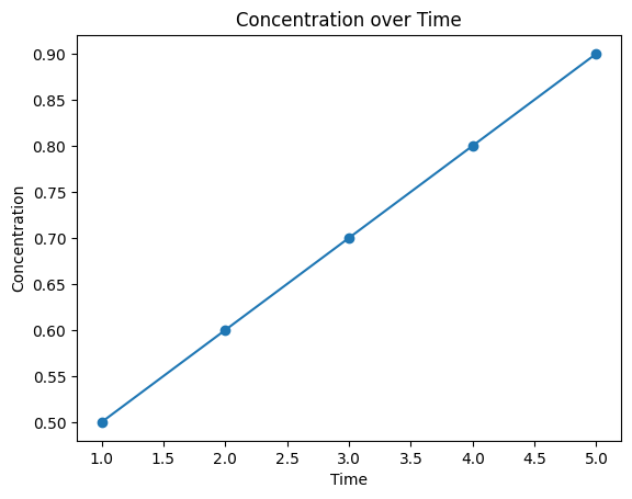
Figure: Line Plot of Time vs. Concentration

Example Code for Scatter Plot:

import seaborn as sns
import pandas as pd

# Load sample dataset
df = pd.DataFrame({'MolecularWeight': [180, 200, 150, 170, 210],
                  'BoilingPoint': [100, 110, 95, 105, 120]})

# Scatter plot
sns.scatterplot(data=df, x='MolecularWeight', y='BoilingPoint')
plt.title('Molecular Weight vs Boiling Point')
plt.show()

Output

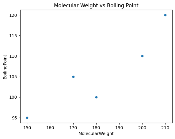
Figure: Scatter Plot of Molecular Weight vs. Boiling Point

Histograms and Density Plots

Explanation:

Histograms display the distribution of a single variable by dividing it into bins, while density plots are smoothed versions of histograms that show the probability density.

Example Code for Histogram:

import matplotlib.pyplot as plt

# Example data
data = [1.1, 2.3, 2.9, 3.5, 4.0, 4.4, 5.1, 5.9, 6.3, 6.8, 7.2, 8.0, 9.1, 9.7, 10.2]

# Create histogram
plt.hist(data, bins=8, edgecolor='black', color='skyblue')
plt.xlabel('Value')
plt.ylabel('Frequency')
plt.title('Histogram Demonstrating Data Distribution')
plt.grid(axis='y', linestyle='--', alpha=0.7)  # Add grid for better readability
plt.show()

Output

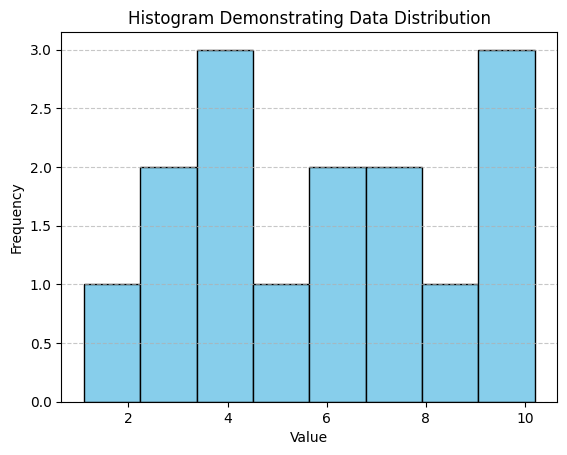
Figure: Histogram Demonstrating Data Distribution

Example Code for Density Plot:

import seaborn as sns

# Example data
data = [1.1, 2.3, 2.9, 3.5, 4.0, 4.4, 5.1, 5.9, 6.3, 6.8, 7.2, 8.0, 9.1, 9.7, 10.2]

# Density plot
sns.kdeplot(data, fill=True)
plt.xlabel('Value')
plt.ylabel('Density')
plt.title('Density Plot')
plt.show()

Output

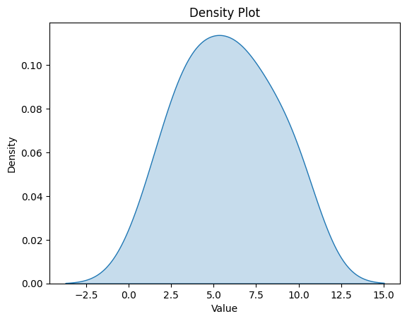
Figure: Density Plot Visualizing Data Distribution

Box Plots and Violin Plots

Explanation: Box plots show the distribution of data based on quartiles and are useful for spotting outliers. Violin plots combine box plots and density plots to provide more detail on the distribution’s shape.

Example Code for Box Plot:

import seaborn as sns
import pandas as pd

# Sample data
df = pd.DataFrame({'Category': ['A', 'A', 'B', 'B', 'C', 'C'],
                  'Value': [10, 15, 10, 20, 15, 25]})

# Box plot
sns.boxplot(data=df, x='Category', y='Value')
plt.title('Box Plot')
plt.show()

Output

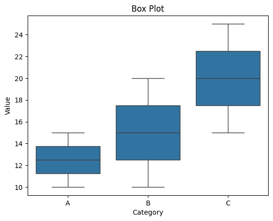
Figure: Box Plot Showing Value Distribution Across Categories

Example Code for Violin Plot:

import seaborn as sns
import pandas as pd

# Sample data
df = pd.DataFrame({'Category': ['A', 'A', 'B', 'B', 'C', 'C'],
                  'Value': [10, 15, 10, 20, 15, 25]})

# Violin plot
sns.violinplot(data=df, x='Category', y='Value')
plt.title('Violin Plot')
plt.show()

Output

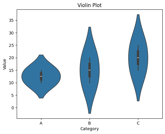
Figure: Violin Plot Highlighting Value Distribution and Density Across Categories

Heatmaps and Correlation Matrices

Explanation: Heatmaps display data as a color-coded matrix. They are often used to show correlations between variables or visualize patterns within data.

Example Code for Heatmap:

import seaborn as sns
import numpy as np
import pandas as pd

# Sample correlation data
data = np.random.rand(5, 5)
df = pd.DataFrame(data, columns=['A', 'B', 'C', 'D', 'E'])

# Heatmap
sns.heatmap(df, annot=True, cmap='coolwarm')
plt.title('Heatmap')
plt.show()

Figure: Heatmap Depicting Data as a Color-Coded Matrix

Example Code for Correlation Matrix:

import seaborn as sns
import numpy as np
import pandas as pd

# Sample correlation data
data = np.random.rand(5, 5)
df = pd.DataFrame(data, columns=['A', 'B', 'C', 'D', 'E'])

# Correlation matrix of a DataFrame
corr_matrix = df.corr()

# Heatmap of the correlation matrix
sns.heatmap(corr_matrix, annot=True, cmap='coolwarm')
plt.title('Correlation Matrix')
plt.show()

Figure: Heatmap Visualizing the Correlation Matrix Across Variables

2.2.6 Statistical Analysis Basics

Completed and Compiled Code: Click Here

Statistical analysis is essential for interpreting data and making informed conclusions. In this section, we’ll explore fundamental statistical techniques using Python, which are particularly useful in scientific research.

Descriptive Statistics

Explanation: Descriptive statistics summarize and describe the main features of a dataset. Common descriptive statistics include the mean, median, mode, variance, and standard deviation.

Example Code:

import pandas as pd

# Load a sample dataset
df = pd.DataFrame({'MolecularWeight': [180, 200, 150, 170, 210],
                  'BoilingPoint': [100, 110, 95, 105, 120]})

# Calculate descriptive statistics
mean_mw = df['MolecularWeight'].mean()
median_bp = df['BoilingPoint'].median()
std_mw = df['MolecularWeight'].std()

print(f"Mean Molecular Weight: {mean_mw}")
print(f"Median Boiling Point: {median_bp}")
print(f"Standard Deviation of Molecular Weight: {std_mw}")

Output

Mean Molecular Weight: 182.0
Median Boiling Point: 105.0
Standard Deviation of Molecular Weight: 23.874672772626646

Practice Problem 1: Calculate the mean, median, and variance for the num column in the BBBP dataset.

▶ Show Solution Code


import pandas as pd

# Load the BBBP dataset
url = 'https://raw.githubusercontent.com/Data-Chemist-Handbook/Data-Chemist-Handbook.github.io/refs/heads/master/_pages/BBBP.csv'
df = pd.read_csv(url)

# Calculate the mean, median, and variance
mean_num = df['num'].mean()
median_num = df['num'].median()
variance_num = df['num'].var()

print(f'Mean: {mean_num}, Median: {median_num}, Variance: {variance_num}')

Output

Mean: 1027.3760975609757, Median: 1026.5, Variance: 351455.5290526015

Probability Distributions

Explanation:

Probability distributions are a fundamental concept in data analysis, representing how values in a dataset are distributed across different ranges. One of the most well-known and frequently encountered probability distributions is the normal distribution (also known as the Gaussian distribution).

The normal distribution is characterized by:

A bell-shaped curve that is symmetric around its mean.
The majority of values clustering near the mean, with fewer values occurring as you move further away.
Its shape is determined by two parameters:
- Mean (μ): The central value where the curve is centered.
- Standard deviation (σ): A measure of the spread of data around the mean. A smaller σ results in a steeper, narrower curve, while a larger σ produces a wider, flatter curve.

In cheminformatics, normal distributions can describe various molecular properties, such as bond lengths, molecular weights, or reaction times, especially when the data arises from natural phenomena or measurements.

Why Normal Distributions Matter for Chemists:

Predicting Properties: A normal distribution can be used to predict probabilities, such as the likelihood of a molecular property (e.g., boiling point) falling within a certain range.
Outlier Detection: Chemists can identify unusual molecular behaviors or experimental measurements that deviate significantly from the expected distribution.
Statistical Modeling: Many statistical tests and machine learning algorithms assume that the data follows a normal distribution.

Example Code for Normal Distribution:

This code generates data following a normal distribution and visualizes it with a histogram:

import numpy as np
import matplotlib.pyplot as plt

# Generate data with a normal distribution
data = np.random.normal(loc=0, scale=1, size=1000)

# Plot the histogram
plt.hist(data, bins=30, density=True, alpha=0.6, color='b')
plt.xlabel('Value')
plt.ylabel('Probability')
plt.title('Normal Distribution')
plt.show()

Output

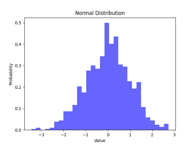
Note: This code can result in a different output every time it is run, since np.random.normal generates random data

What the Code Does:

Generate Data: The np.random.normal function creates 1000 random data points with:
- Mean (loc): Set to 0.
- Standard Deviation (scale): Set to 1.
Plot Histogram: The plt.hist function divides the data into 30 equal-width bins and plots a histogram:
- density=True ensures the histogram represents a probability density function (area under the curve sums to 1).
- alpha=0.6 adjusts the transparency of the bars.
- color='b' specifies the bar color as blue.
Labels and Title: The axes are labeled for clarity, and the title describes the chart.

Interpretation:

The plot shows the majority of values concentrated around 0 (the mean), with the frequency tapering off symmetrically on either side.
The shape of the curve reflects the standard deviation. Most values (approximately 68%) fall within one standard deviation (μ±σ) of the mean.

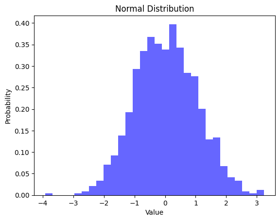
Figure: Histogram Depicting a Normal Distribution with Mean 0 and Standard Deviation 1

Applications in Chemistry:

Molecular Property Analysis: Understand the variation in molecular weights or boiling points for a compound set.
Error Analysis: Model and visualize experimental errors, assuming they follow a normal distribution.
Kinetic Studies: Analyze reaction times or rates for processes that exhibit natural variability.

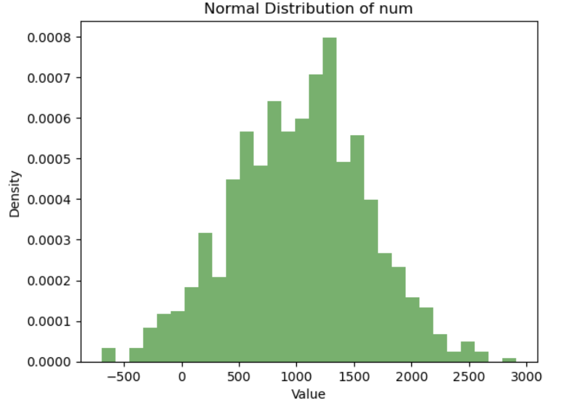
Practice Problem 2: Generate a normally distributed dataset based on the mean and standard deviation of the num column in the BBBP dataset. Plot a histogram of the generated data.

▶ Show Solution Code


import pandas as pd
import numpy as np
import matplotlib.pyplot as plt

# Load the BBBP dataset
url = 'https://raw.githubusercontent.com/Data-Chemist-Handbook/Data-Chemist-Handbook.github.io/refs/heads/master/_pages/BBBP.csv'
df = pd.read_csv(url)

# Generate normally distributed data based on 'num' column
mean_num = df['num'].mean()
std_num = df['num'].std()
normal_data = np.random.normal(mean_num, std_num, size=1000)

# Plot histogram
plt.hist(normal_data, bins=30, density=True, alpha=0.6, color='g')
plt.xlabel('Value')
plt.ylabel('Density')
plt.title('Normal Distribution of num')
plt.show()

Output

Hypothesis Testing

Explanation:

Hypothesis testing is a statistical method used to evaluate whether there is enough evidence in a sample to infer a condition about a population. It is widely used in experimental chemistry to compare groups and draw conclusions about the effects of different treatments or conditions.

Key Concepts:

Null and Alternative Hypotheses:
- Null Hypothesis (H₀): Assumes no difference between the groups being tested (e.g., the means of two groups are equal).
- Alternative Hypothesis (Hₐ): Assumes there is a difference between the groups (e.g., the means of two groups are not equal).
T-Test:
- A t-test compares the means of two independent groups to determine if the observed differences are statistically significant.
- It calculates a t-statistic and a p-value to assess the evidence against the null hypothesis.
Interpreting Results:
- T-Statistic: Measures the difference between group means relative to the variability of the data. Larger values suggest greater differences.
- P-Value: Represents the probability of observing the data assuming H₀ is true. A small p-value (commonly < 0.05) indicates significant differences between groups.
Why It’s Useful for Chemists:
- Compare reaction yields under different conditions (e.g., catalysts or solvents).
- Evaluate the effectiveness of a new material or treatment compared to a control group.

Example Code for t-test:

from scipy.stats import ttest_ind
import pandas as pd

# Example data
group_a = [1.2, 2.3, 1.8, 2.5, 1.9]  # Results for treatment A
group_b = [2.0, 2.1, 2.6, 2.8, 2.4]  # Results for treatment B

# Perform t-test
t_stat, p_val = ttest_ind(group_a, group_b)
print(f"T-statistic: {t_stat}, P-value: {p_val}")

Output

T-statistic: -1.6285130624347315, P-value: 0.14206565386214137

What the Code Does:

Data Input:
- group_a and group_b contain measurements from two independent groups (e.g., yields from two catalysts).
T-Test Execution:
- The ttest_ind() function performs an independent two-sample t-test to compare the means of the two groups.
Output:
- T-Statistic: Quantifies the difference in means relative to data variability.
- P-Value: Indicates whether the observed difference is statistically significant.

Interpretation:

The t-statistic is -1.63, indicating that the mean of group_a is slightly lower than the mean of group_b.
The p-value is 0.14, which is greater than 0.05. This means we fail to reject the null hypothesis and conclude that there is no statistically significant difference between the two groups.

Applications in Chemistry:

Catalyst Comparison:
- Determine if two catalysts produce significantly different yields or reaction rates.
Material Testing:
- Evaluate whether a new material significantly improves a property (e.g., tensile strength, thermal stability) compared to a standard material.
Experimental Conditions:
- Test whether changes in temperature, pressure, or solvent lead to meaningful differences in reaction outcomes.

Important Considerations:

Ensure the data meets the assumptions of a t-test:
- Independence of groups.
- Approximately normal distribution.
- Similar variances (use Welch’s t-test if variances differ).
For multiple group comparisons, consider using ANOVA instead of a t-test.

By using hypothesis testing, chemists can make statistically supported decisions about experimental results and conditions.

Practice Problem 3: In the BBBP dataset, compare the mean num values between permeable (p_np=1) and non-permeable (p_np=0) compounds using a t-test.

▶ Show Solution Code


from scipy.stats import ttest_ind
import pandas as pd

# Load the BBBP dataset
url = 'https://raw.githubusercontent.com/Data-Chemist-Handbook/Data-Chemist-Handbook.github.io/refs/heads/master/_pages/BBBP.csv'
df = pd.read_csv(url)

# Separate data by permeability
permeable = df[df['p_np'] == 1]['num']
non_permeable = df[df['p_np'] == 0]['num']

# Perform t-test
t_stat, p_val = ttest_ind(permeable, non_permeable)
print(f"T-statistic: {t_stat}, P-value: {p_val}")

Output

Correlation and Regression

Explanation:

Correlation and regression are statistical tools used to analyze relationships between variables. These methods are crucial for chemists to understand how different molecular properties are related and to make predictions based on data.

Correlation:

Definition: Correlation quantifies the strength and direction of a linear relationship between two variables.
Range: The correlation coefficient (r) ranges from -1 to 1:
- r = 1: Perfect positive correlation (as one variable increases, the other also increases proportionally).
- r = -1: Perfect negative correlation (as one variable increases, the other decreases proportionally).
- r = 0: No correlation.
Use in Chemistry: For example, correlation can reveal whether molecular weight is related to boiling point in a set of compounds.

Regression:

Definition: Regression predicts the value of a dependent variable based on one or more independent variables.
Types: Simple linear regression (one independent variable) and multiple linear regression (two or more independent variables).
Output:
- Regression Coefficient (β): Indicates the magnitude and direction of the relationship between the independent variable and the dependent variable.
- Intercept (α): Represents the predicted value of the dependent variable when the independent variable is zero.
- Use in Chemistry: Regression can predict molecular properties, such as boiling point, based on easily measurable features like molecular weight.

Example Code for Correlation and Linear Regression:

import pandas as pd
import seaborn as sns
from scipy.stats import pearsonr
from sklearn.linear_model import LinearRegression

# Example data
df = pd.DataFrame({'MolecularWeight': [180, 200, 150, 170, 210],
                  'BoilingPoint': [100, 110, 95, 105, 120]})

# Calculate correlation
corr, _ = pearsonr(df['MolecularWeight'], df['BoilingPoint'])
print(f"Correlation: {corr}")

# Linear regression
X = df[['MolecularWeight']]  # Independent variable
y = df['BoilingPoint']       # Dependent variable
model = LinearRegression().fit(X, y)

# Regression results
print(f"Regression coefficient: {model.coef_[0]}")
print(f"Intercept: {model.intercept_}")

Output

Correlation: 0.9145574682496187
Regression coefficient: 0.36842105263157904
Intercept: 38.947368421052616

What the Code Does:

Input Data:
- The DataFrame contains molecular weight and boiling point values for five molecules.
Correlation:
- The pearsonr function calculates the Pearson correlation coefficient (r) between molecular weight and boiling point.
- Example output: If r = 0.95, it indicates a strong positive linear relationship.
Regression:
- The LinearRegression class models the relationship between molecular weight (independent variable) and boiling point (dependent variable).
- Key Outputs:
  - Regression Coefficient: Shows how much the boiling point changes for a one-unit increase in molecular weight.
  - Intercept: Indicates the boiling point when the molecular weight is zero.

Interpretation:

If the correlation coefficient is high (close to 1 or -1), it suggests a strong linear relationship.
The regression coefficient quantifies the strength of this relationship, and the intercept gives the baseline prediction.

Applications in Chemistry:

Molecular Property Prediction:
- Predict boiling points of new compounds based on molecular weight or other properties.
Quantitative Structure-Property Relationships (QSPR):
- Use regression to model how structural features influence chemical properties like solubility or reactivity.
Experimental Design:
- Understand relationships between variables to guide targeted experiments.

Practice Problem 4: Calculate the correlation between num and p_np in the BBBP dataset. Then, perform a linear regression to predict num based on p_np.

▶ Show Solution Code


import pandas as pd
from scipy.stats import pearsonr
from sklearn.linear_model import LinearRegression

# Load the BBBP dataset
url = 'https://raw.githubusercontent.com/Data-Chemist-Handbook/Data-Chemist-Handbook.github.io/refs/heads/master/_pages/BBBP.csv'
df = pd.read_csv(url)

# Calculate correlation
corr, _ = pearsonr(df['num'], df['p_np'])
print(f"Correlation between num and p_np: {corr}")

# Linear regression
X = df[['p_np']]
y = df['num']
model = LinearRegression().fit(X, y)
print(f"Regression coefficient: {model.coef_[0]}")
print(f"Intercept: {model.intercept_}")

Output

Correlation between num and p_np: 0.43004111834348224
Regression coefficient: 600.5995724446169
Intercept: 568.2836438923343

ANOVA (Analysis of Variance)

Explanation:

ANOVA (Analysis of Variance) is a statistical method used to determine if there are significant differences between the means of three or more independent groups. It helps chemists evaluate whether variations in a continuous variable (e.g., melting point or reaction yield) are influenced by a categorical variable (e.g., types of catalysts or reaction conditions).

Key Concepts:

Groups and Variability:
- ANOVA compares the variability within each group to the variability between groups.
- If the variability between groups is significantly larger than the variability within groups, it suggests that the group means are different.
Hypotheses:
- Null Hypothesis (H₀): All group means are equal.
- Alternative Hypothesis (Hₐ): At least one group mean is different.
F-Statistic:
- The F-statistic is calculated as the ratio of between-group variability to within-group variability.
- A larger F-statistic indicates a greater likelihood of differences between group means.
P-Value:
- The p-value indicates the probability of observing the F-statistic if H₀ is true.
- A small p-value (typically < 0.05) leads to rejecting H₀, suggesting that group means are significantly different.

Why It’s Useful for Chemists:

ANOVA can identify whether different conditions (e.g., catalysts, solvents, or temperatures) significantly affect a property of interest, such as yield, rate, or stability.

Example Code for ANOVA:

from scipy.stats import f_oneway

# Example data for three groups
group1 = [1.1, 2.2, 3.1, 2.5, 2.9]  # Data for condition 1
group2 = [2.0, 2.5, 3.5, 2.8, 3.0]  # Data for condition 2
group3 = [3.1, 3.5, 2.9, 3.6, 3.3]  # Data for condition 3

# Perform ANOVA
f_stat, p_val = f_oneway(group1, group2, group3)
print(f"F-statistic: {f_stat}, P-value: {p_val}")

Output:

F-statistic: 3.151036525172754, P-value: 0.07944851235243751

What the Code Does:

Data Input:
- Three groups of data represent different experimental conditions (e.g., three catalysts tested for their effect on reaction yield).
ANOVA Test:
- The f_oneway() function performs a one-way ANOVA test to determine if there are significant differences between the group means.
Results:
- F-Statistic: Measures the ratio of between-group variability to within-group variability.
- P-Value: If this is below a threshold (e.g., 0.05), it suggests that the differences in means are statistically significant.

Interpretation:

The p-value (0.08) is greater than 0.05, so we cannot reject the null hypothesis.
This indicates that it isn’t statistically significant from the others.

Applications in Chemistry:

Catalyst Screening:
- Compare reaction yields across multiple catalysts to identify the most effective one.
Reaction Optimization:
- Evaluate the effect of different temperatures, solvents, or reaction times on product yield or purity.
Material Properties:
- Analyze differences in tensile strength or thermal stability across materials produced under different conditions.
Statistical Quality Control:
- Assess variability in product quality across batches.

By using ANOVA, chemists can draw statistically sound conclusions about the effects of categorical variables on continuous properties, guiding decision-making in experimental designs.

Practice Problem 5: Group the num column in the BBBP dataset by the first digit of num (e.g., 1XX, 2XX, 3XX) and perform an ANOVA test to see if the mean values differ significantly among these groups.

▶ Show Solution Code


from scipy.stats import f_oneway
import pandas as pd

# Load the BBBP dataset
url = 'https://raw.githubusercontent.com/Data-Chemist-Handbook/Data-Chemist-Handbook.github.io/refs/heads/master/_pages/BBBP.csv'
df = pd.read_csv(url)

# Group 'num' by the first digit
group1 = df[df['num'].between(100, 199)]['num']
group2 = df[df['num'].between(200, 299)]['num']
group3 = df[df['num'].between(300, 399)]['num']

# Perform ANOVA
f_stat, p_val = f_oneway(group1, group2, group3)
print(f"F-statistic: {f_stat}, P-value: {p_val}")

Output

Section 2.2 – Quiz Questions

Explanation: `astype()` is used to convert a column's data type, such as from string to float or integer, so mathematical operations can be performed.

2) Comprehension / Application Questions

Question 6

You have just received a dataset regarding the toxicity of commonly used compounds (TOX21) and would like to get an idea of the metrics in the dataset.

Task: Read the TOX21.csv dataset into a DataFrame and print the first five rows. Which of the following matches your third compound in the output?

A. Diethyl oxalate
B. Dimethyl dihydrogen diphosphate
C. Dimethylglyoxime
D. 4’-Methoxyacetophenone

▶ Click to show answer

Correct Answer: C

▶ Click to show explanation

Explanation: The third row of the dataset contains Dimethylglyoxime, based on the output of `df.head()`.

▶ Show Solution Code


import pandas as pd

url = "https://raw.githubusercontent.com/Data-Chemist-Handbook/Data-Chemist-Handbook.github.io/refs/heads/master/_pages/Chemical%20List%20tox21sl-2025-02-20.csv"
df = pd.read_csv(url)
print(df.head())

Question 7

After looking at the TOX21 dataset, you realize that there are missing values in rows and duplicate rows.
To fix this problem, you should handle the missing values by using ___ and get rid of duplicate rows by ___.

A. df.fillna('unknown', inplace=True), df.drop_duplicates()
B. df.fillna(0, inplace=False), df.drop_duplicates(inplace=True)
C. df.dropna(inplace=True), df.drop_duplicates()
D. df.fillna('missing', inplace=True), df.drop_duplicates(inplace=True)

▶ Click to show answer

Correct Answer: A

▶ Click to show explanation

Explanation: `fillna('unknown')` fills missing values with a placeholder, maintaining the dataset's size. `drop_duplicates()` removes any repeated rows to ensure clean data.

Question 8

Which function and code would allow you to create a new column that represents the average of the boiling points 'bp' in your dataset?

A. Grouping; df['avg_bp'] = df['bp'].mean()
B. Grouping; df['avg_bp'] = df['bp'].sum() / len(df)
C. Merging; df['avg_bp'] = df['bp'].apply(lambda x: sum(x) / len(x))
D. Merging; df['avg_bp'] = df.apply(lambda row: row['bp'].mean(), axis=1)

▶ Click to show answer

Correct Answer: A

▶ Click to show explanation

Explanation: The `.mean()` method calculates the column-wise average, and assigning it to a new column applies that single value across all rows.

Question 9

You want to perform an ANOVA statistical analysis to evaluate the activity of the compounds listed in the TOX21 dataset.

Task:
Determine whether the average molecular mass of compounds with ToxCast Active Ratio above 20% is statistically different from those below 20%.

Use a 95% confidence level (α = 0.05).
Calculate the F-statistic and P-value to assess significance.

Question:
Are these two groups statistically significant at the 95% confidence level? What are the F-statistic and P-value?

A. Yes, F-Statistic: 203.89, P-Value: 0.03
B. Yes, F-Statistic: 476.96, P-Value: 0.00
C. No, F-Statistic: 78.09, P-Value: 0.09
D. No, F-Statistic: 548.06, P-Value: 0.10

▶ Click to show answer

Correct Answer: B

▶ Click to show explanation

Explanation: Since the P-value < 0.05, the result is statistically significant at the 95% confidence level. This means the difference in average molecular mass between compounds with high and low ToxCast activity is unlikely due to random chance.

▶ Show Solution Code


import pandas as pd
from scipy.stats import f_oneway

# Load dataset
url = "https://raw.githubusercontent.com/Data-Chemist-Handbook/Data-Chemist-Handbook.github.io/refs/heads/master/_pages/Chemical%20List%20tox21sl-2025-02-20.csv"
df = pd.read_csv(url)

# Clean and prepare data
df = df[['% ToxCast Active', 'AVERAGE MASS']].dropna()
df['toxcast_active_ratio'] = df['% ToxCast Active'] / 100
df['mass'] = df['AVERAGE MASS']

# Define two groups based on active ratio threshold
group_low  = df[df['toxcast_active_ratio'] <= 0.2]['mass']
group_high = df[df['toxcast_active_ratio'] >  0.2]['mass']

# Perform ANOVA
f_stat, p_val = f_oneway(group_low, group_high)

print(f"F-statistic: {f_stat:.2f}")
print(f"P-value:      {p_val:.4f}")

Question 10

You are analyzing a SMILES dataset of drug candidates and want to estimate the carbon atom count for each compound to study how size influences permeability. What code snippet would achieve this?

A. df['carbon_count'] = df['name'].count('C')
B. df['carbon_count'] = df['smiles'].apply(lambda x: x.count('C'))
C. df['carbon_count'] = df['smiles'].sum('C')
D. df['carbon_count'] = count(df['smiles'], 'C')

▶ Click to show answer

Correct Answer: B

▶ Click to show explanation

Explanation: Using `apply()` with a lambda function allows you to count the number of carbon atoms (`'C'`) in each SMILES string.

Question 11

After calculating the carbon counts, you want to see if permeable compounds (p_np = 1) tend to have different carbon counts than non-permeable ones (p_np = 0). Which of the following code snippets best performs this comparison?

A. df.groupby('carbon_count')['p_np'].mean()
B. df.groupby('p_np')['carbon_count'].mean()
C. df.groupby('carbon_count')['p_np'].count()
D. df['carbon_count'].groupby(df['p_np']).sum()

▶ Click to show answer

Correct Answer: B

▶ Click to show explanation

Explanation: Grouping by `'p_np'` and calculating the mean of `'carbon_count'` lets you compare average carbon counts between permeability classes.

Question 12

You want to build a simple model that predicts whether a compound is permeable based on its carbon count. Which two Python tools would best help you analyze the relationship and build a linear model?

A. groupby() and melt()
B. pearsonr() and LinearRegression()
C. pivot_table() and df.fillna()
D. apply() and get_dummies()

▶ Click to show answer

**Correct Answer:** B

▶ Click to show explanation

`pearsonr()` helps determine correlation, while `LinearRegression()` can fit a model to predict one variable based on another.

2.3 Representation

In the realm of cheminformatics and computational chemistry, the representation of chemical compounds is a fundamental aspect that enables the analysis, simulation, and prediction of chemical properties and behaviors. This chapter delves into various methods of representing chemical structures, each with its unique advantages and applications.

Chemical representations serve as the bridge between the abstract world of chemical structures and the computational tools used to analyze them. These representations allow chemists and researchers to encode complex molecular information into formats that can be easily manipulated and interpreted by computers.

This chapter will explore each of these representation methods in detail, providing insights into their applications, strengths, and limitations. By understanding these representations, you will be equipped to leverage computational tools effectively in your chemical research and development endeavors.

2.3.1 SMILES (Simplified Molecular Input Line Entry System)

Completed and Compiled Code: Click Here

Explanation:

SMILES, or Simplified Molecular Input Line Entry System, is a notation that represents molecular structures as text strings. Many sets of rules apply to SMILES formation and interpretation, and these rules have generally become standardized since the development of SMILES in the 1980s. It is a widely used format in cheminformatics due to its simplicity and human-readability. SMILES strings represent atoms and bonds in a molecule, allowing for easy storage and manipulation of chemical information in databases and software applications.

Atoms: Atoms are represented by their atomic symbol either as itself or in brackets. Atoms that do not require brackets must be part of the organic subset of atoms including B, C, N, O, P, S, F, Cl, Br, or I. Within this subset, brackets may still be needed for an atom that is not the most abundant isotope, has a charge, has abnormal valence, or is a chiral center. Hydrogens are usually implied and not listed explicitly, assuming normal valence.
Bonds: Single bonds are implied between atoms adjacent in the string, while double, triple, and aromatic bonds are represented by ‘=’, ‘#’, and ‘:’ respectively.
Branches: Branched molecules use parentheses around subordinate branched groups to indicate branching in the molecular structure.
Rings: Rings are represented with numbers that indicate the atoms at the start and end of a ring, with the digit following after the letter symbol of the atoms. Usually the same number is used to identify the ring start and finish to distinguish between multiple rings. For example, cyclohexane would be written as C1CCCCC1 and napthalene can be written as c1c2ccccc2ccc1 (SMILES are not case sensitive)

Importance and Applications:

SMILES is crucial for cheminformatics because it provides a compact and efficient way to represent chemical structures in a text format. This makes it ideal for storing large chemical databases, transmitting chemical information over the internet, and integrating with various software tools. SMILES is used in drug discovery, chemical informatics, and molecular modeling to facilitate the exchange and analysis of chemical data. For example, pharmaceutical companies use SMILES to store and retrieve chemical structures in their databases, enabling rapid screening of potential drug candidates.

Case Study:

Context: A pharmaceutical company is developing a new drug and needs to screen a large library of chemical compounds to identify potential candidates. By using SMILES notation, they can efficiently store and manage the chemical structures in their database.

Application: The company uses SMILES to encode the structures of thousands of compounds. They then apply cheminformatics tools to perform virtual screening, identifying compounds with desired properties and filtering out those with undesirable characteristics. This process significantly accelerates the drug discovery pipeline by narrowing down the list of potential candidates for further testing.

Example Code:

// you have to import the package in a separate code cell
!pip install rdkit-pypi

import pandas as pd
from rdkit import Chem

# Example SMILES string for Aspirin
smiles = 'CC(=O)OC1=CC=CC=C1C(=O)O'

# Convert SMILES to a molecule object
molecule = Chem.MolFromSmiles(smiles)

# Display basic information about the molecule
print("Number of atoms:", molecule.GetNumAtoms())
print("Number of bonds:", molecule.GetNumBonds())

# Example of using iloc to access the first element in a DataFrame column
# Create a simple DataFrame
data = {'smiles': ['CC(=O)OC1=CC=CC=C1C(=O)O', 'C1=CC=CC=C1']}
df = pd.DataFrame(data)

# Access the first SMILES string using iloc
first_smiles = df['smiles'].iloc[0]
print("First SMILES string:", first_smiles)

# Identify aromatic rings using GetSymmSSSR
aromatic_rings = [ring for ring in Chem.GetSymmSSSR(molecule) if all(molecule.GetAtomWithIdx(atom).GetIsAromatic() for atom in ring)]
print("Number of aromatic rings:", len(aromatic_rings))

Output

Number of atoms: 13
Number of bonds: 13
First SMILES string: CC(=O)OC1=CC=CC=C1C(=O)O
Number of aromatic rings: 1

What the Code Does

SMILES Conversion to Molecule Object:
- The SMILES (Simplified Molecular Input Line Entry System) string CC(=O)OC1=CC=CC=C1C(=O)O represents Aspirin.

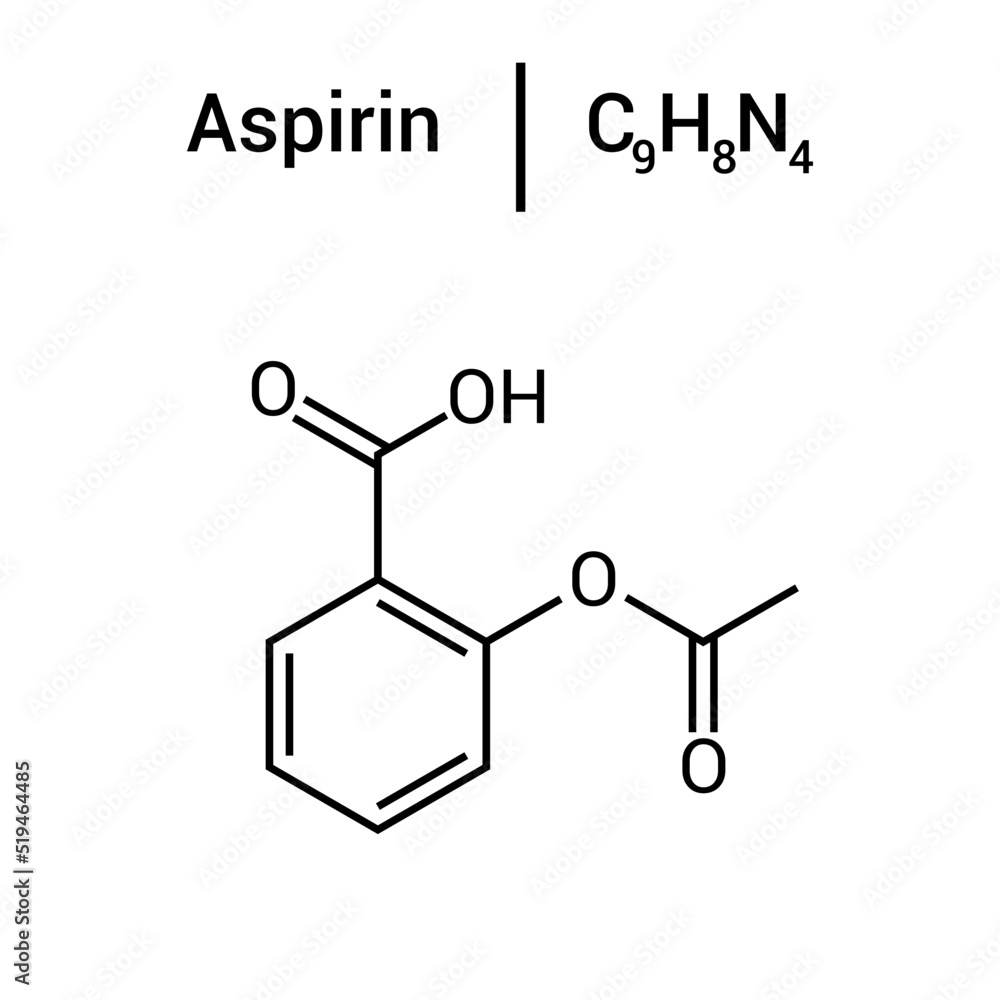
Chem.MolFromSmiles(smiles) converts the SMILES string into an RDKit molecule object, allowing further chemical analysis.

Basic Molecular Properties:
- GetNumAtoms() retrieves the total number of atoms in the molecule.
- GetNumBonds() retrieves the total number of bonds in the molecule.
DataFrame Creation and Data Access:
- A DataFrame df is created with a column smiles, containing two SMILES strings.
- iloc[0] accesses the first SMILES string in the smiles column.
Identification of Aromatic Rings:
- Chem.GetSymmSSSR(molecule) identifies all rings in the molecule.
- The list comprehension filters out aromatic rings by checking if all atoms in a ring are aromatic (GetIsAromatic()).
Output Results:
- The code outputs:
- The number of atoms and bonds in the molecule.
- The first SMILES string from the DataFrame.
- The number of aromatic rings in the molecule.

Interpretation

Practical Application:
This code is useful for chemical informatics tasks such as analyzing molecular structures, detecting aromaticity, and managing chemical data in tabular formats.
Use Case:
Researchers can use this script for analyzing molecular properties, storing chemical datasets in DataFrames, and identifying features like aromaticity for further studies.

Practice Problem:

Context: SMILES notation is a powerful tool for representing chemical structures. Understanding how to convert SMILES strings into molecular objects and extract information is crucial for cheminformatics applications.

Task: Using the BBBP.csv dataset, write Python code to:

Read the dataset and extract the SMILES strings.
Convert the first SMILES string into a molecule object using RDKit.
Print the number of atoms and bonds in the molecule.
Identify and print the aromatic rings in the molecule.

Solution:

import pandas as pd
from rdkit import Chem

# Load the BBBP dataset
url = 'https://raw.githubusercontent.com/Data-Chemist-Handbook/Data-Chemist-Handbook.github.io/refs/heads/master/_pages/BBBP.csv'
df = pd.read_csv(url)

# Extract the first SMILES string
first_smiles = df['smiles'].iloc[0]

# Convert SMILES to a molecule object
molecule = Chem.MolFromSmiles(first_smiles)

# Print the number of atoms and bonds
print("Number of atoms:", molecule.GetNumAtoms())
print("Number of bonds:", molecule.GetNumBonds())

# Identify aromatic rings
aromatic_rings = [ring for ring in Chem.GetSymmSSSR(molecule) if all(molecule.GetAtomWithIdx(atom).GetIsAromatic() for atom in ring)]
print("Number of aromatic rings:", len(aromatic_rings))

Output

Number of atoms: 20
Number of bonds: 20
Number of aromatic rings: 2

Explanation: This code loads the BBBP dataset and analyzes the first molecule by extracting its SMILES (Simplified Molecular Input Line Entry System) string, which is a text-based representation of its structure. It then converts that string into an RDKit molecule object to examine its properties. The output — number of atoms, bonds, and aromatic rings — describes the first molecule in the dataset, without applying any additional filters or conditions. The line identifying aromatic rings uses a list comprehension to find all rings in the molecule where every atom is aromatic. In short, the code gives a basic structural overview of the very first compound in the BBBP dataset.

2.3.2 SMARTS (SMILES Arbitrary Target Specification)

Completed and Compiled Code: Click Here

Explanation:

SMARTS, or SMILES Arbitrary Target Specification, is an extension of the SMILES notation used to define substructural patterns in molecules. It is particularly useful in cheminformatics for searching and matching specific molecular features within large chemical databases. SMARTS allows for more complex queries than SMILES by incorporating logical operators and wildcards to specify atom and bond properties.

Atoms and Bonds: Similar to SMILES, but with additional symbols to specify atom and bond properties.
Logical Operators: Used to define complex patterns, such as ‘and’, ‘or’, and ‘not’.
Wildcards: Allow for flexible matching of atom types and bond orders.

Importance and Applications:

SMARTS is essential for cheminformatics because it enables the identification and extraction of specific substructures within molecules. This capability is crucial for tasks such as virtual screening, lead optimization, and structure-activity relationship (SAR) studies. SMARTS is widely used in drug discovery to identify potential pharmacophores and optimize chemical libraries. For instance, researchers can use SMARTS to search for molecules containing specific functional groups that are known to interact with biological targets.

Case Study:

Context: A research team is investigating a class of compounds known to inhibit a specific enzyme. They need to identify compounds in their database that contain a particular substructure associated with enzyme inhibition.

Application: The team uses SMARTS to define the substructural pattern of interest. By applying this SMARTS pattern to their chemical database, they can quickly identify and extract compounds that match the pattern. This targeted approach allows them to focus their experimental efforts on compounds with the highest likelihood of success, saving time and resources.

Example Code:

!pip install rdkit-pypi

import pandas as pd
from rdkit import Chem

# Example SMARTS pattern for an aromatic ring
smarts = 'c1ccccc1'

# Convert SMARTS to a molecule pattern
pattern = Chem.MolFromSmarts(smarts)

# Example molecule (Benzene)
benzene_smiles = 'C1=CC=CC=C1'
benzene = Chem.MolFromSmiles(benzene_smiles)

# Check if the pattern matches the molecule
match = benzene.HasSubstructMatch(pattern)
print("Does the molecule match the SMARTS pattern?", match)

# Example of using iloc to access the first element in a DataFrame column
# Create a simple DataFrame
data = {'smiles': ['C1=CC=CC=C1', 'C1=CC=CN=C1']}
df = pd.DataFrame(data)

# Access the first SMILES string using iloc
first_smiles = df['smiles'].iloc[0]
print("First SMILES string:", first_smiles)

Output

Does the molecule match the SMARTS pattern? True
First SMILES string: C1=CC=CC=C1

What the Code Does:

SMARTS Pattern Definition:
- SMARTS (SMiles ARbitrary Target Specification) is a syntax for describing substructure patterns.
- The SMARTS string c1ccccc1 represents a simple aromatic ring, such as benzene.
Conversion to Molecule Pattern:
- Chem.MolFromSmarts(smarts) converts the SMARTS string into a molecule pattern object, which can be used for substructure matching.
SMILES Conversion to Molecule Object:
- The SMILES (Simplified Molecular Input Line Entry System) string C1=CC=CC=C1 represents benzene.
- Chem.MolFromSmiles(benzene_smiles) converts this string into an RDKit molecule object for further analysis.
Substructure Matching:
- benzene.HasSubstructMatch(pattern) checks if the benzene molecule contains the substructure defined by the SMARTS pattern. The result is True because benzene is an aromatic ring.
DataFrame Creation and Data Access:
- A DataFrame df is created with a column smiles, containing two SMILES strings.
- iloc[0] accesses the first SMILES string in the smiles column.
Output Results:
- Whether the benzene molecule matches the SMARTS pattern.
- The first SMILES string from the DataFrame.

Practice Problem 1:

Context: SMARTS notation is a powerful tool for identifying specific substructures within molecules. Understanding how to use SMARTS to search for patterns is crucial for cheminformatics applications.

Task: Using the BBBP.csv dataset, write Python code to:

Read the dataset and extract the SMILES strings.
Define a SMARTS pattern to identify molecules containing an amine group (N).
Count how many molecules in the dataset match this pattern.

Solution:

import pandas as pd
from rdkit import Chem
from rdkit import RDLogger

# Suppress RDKit warnings
RDLogger.DisableLog('rdApp.*')

# Load the BBBP dataset
url = 'https://raw.githubusercontent.com/Data-Chemist-Handbook/Data-Chemist-Handbook.github.io/refs/heads/master/_pages/BBBP.csv'
df = pd.read_csv(url)

# Define a SMARTS pattern for an amine group
amine_smarts = '[NX3;H2,H1;!$(NC=O)]'
amine_pattern = Chem.MolFromSmarts(amine_smarts)

# Count molecules with an amine group
amine_count = 0
for smiles in df['smiles']:
    molecule = Chem.MolFromSmiles(smiles)
    if molecule is not None and molecule.HasSubstructMatch(amine_pattern):
        amine_count += 1

print("Number of molecules with an amine group:", amine_count)

Output

Number of molecules with an amine group: 555

This section provides a comprehensive overview of SMARTS, including its syntax, advantages, and practical applications in cheminformatics. The example code, practice problem, and solution demonstrate how to work with SMARTS using RDKit, a popular cheminformatics toolkit, and leverage real data from the BBBP dataset.

2.3.3 Fingerprint

Completed and Compiled Code: Click Here

Explanation:

Fingerprints are a type of molecular representation that encodes the presence or absence of certain substructures within a molecule as a binary or hexadecimal string. They are widely used in cheminformatics for tasks such as similarity searching, clustering, and classification of chemical compounds. Fingerprints provide a compact and efficient way to represent molecular features, making them ideal for large-scale database searches.

Types of Fingerprints:
Structural Fingerprints: Represent specific substructures or fragments within a molecule.
Topological Fingerprints: Capture the connectivity and arrangement of atoms in a molecule.
Pharmacophore Fingerprints: Encode the spatial arrangement of features important for biological activity.

Importance and Applications:

Fingerprints are crucial for cheminformatics because they enable the rapid comparison of molecular structures. This capability is essential for tasks such as virtual screening, chemical clustering, and similarity searching. Fingerprints are widely used in drug discovery to identify compounds with similar biological activities and to explore chemical space efficiently. For example, researchers can use fingerprints to quickly identify potential drug candidates that share structural similarities with known active compounds.

Case Study:

Context: A biotech company is developing a new class of antibiotics and needs to identify compounds with similar structures to a known active compound.

Application: The company generates fingerprints for their library of chemical compounds and the known active compound. By comparing the fingerprints, they can quickly identify compounds with similar structural features. This approach allows them to prioritize compounds for further testing, increasing the efficiency of their drug development process.

Example Code:

from rdkit import Chem
from rdkit.Chem import rdFingerprintGenerator

# Example SMILES string for Aspirin
smiles = 'CC(=O)OC1=CC=CC=C1C(=O)O'

# Convert SMILES to a molecule object
molecule = Chem.MolFromSmiles(smiles)

# Use the Morgan fingerprint generator
generator = rdFingerprintGenerator.GetMorganGenerator(radius=2, fpSize=128)
fingerprint = generator.GetFingerprint(molecule)

# Display the fingerprint as a bit string
print("Fingerprint:", fingerprint.ToBitString())

Output

Fingerprint: 00100100001101000000000100000000010000010000000100100001000010001100000110000000110000100000000000001000000000010000000001000100

What the Code Does

SMILES to Molecule Conversion:
- The SMILES (Simplified Molecular Input Line Entry System) string ‘CC(=O)OC1=CC=CC=C1C(=O)O’ represents Aspirin.
- Chem.MolFromSmiles(smiles) converts the SMILES string into an RDKit molecule object that can be processed computationally.
Fingerprint Generator Initialization:
- rdFingerprintGenerator.GetMorganGenerator(radius=2, fpSize=128) initializes a Morgan fingerprint generator with:
- radius=2: Defines the number of bond hops from each atom to consider when generating substructure patterns. (Common values: 2 (ECFP4), 3 (ECFP6), where the number represents the radius)
- fpSize=128: The fingerprint is compressed into a 128-bit vector, which is shorter than the default 1024-bit vector, making it more compact. (Typical sizes: 128, 256, 512, 1024, 2048)
Fingerprint Generation:
- generator.GetFingerprint(molecule) computes the circular fingerprint (Morgan fingerprint) of the molecule. This captures topological information about atom environments, encoding structural features into a binary format.
Fingerprint Representation:
- fingerprint.ToBitString() converts the binary fingerprint into a readable string of 0s and 1s.
- This 128-bit string can be used for molecular similarity, clustering, or as input features for machine learning models in cheminformatics.

Practice Problem 1:

Context: Fingerprints are essential for comparing molecular structures and identifying similar compounds. Understanding how to generate and use fingerprints is crucial for cheminformatics applications.

Task: Using the BBBP.csv dataset, write Python code to:

Read the dataset and extract the SMILES strings.
Generate Morgan fingerprints for the first five molecules.
Print the fingerprints as bit strings.

Solution:

from rdkit import Chem
from rdkit.Chem import rdFingerprintGenerator
import pandas as pd

# Load the BBBP dataset
url = 'https://raw.githubusercontent.com/Data-Chemist-Handbook/Data-Chemist-Handbook.github.io/refs/heads/master/_pages/BBBP.csv'
df = pd.read_csv(url)

# Initialize the Morgan fingerprint generator
generator = rdFingerprintGenerator.GetMorganGenerator(radius=2, fpSize=20)  # You can increase fpSize

# Generate Morgan fingerprints for the first five molecules
for i in range(5):
    smiles = df['smiles'].iloc[i]
    molecule = Chem.MolFromSmiles(smiles)
    fingerprint = generator.GetFingerprint(molecule)
    print(f"Fingerprint for molecule {i+1}:", fingerprint.ToBitString())

Output

Fingerprint for molecule 1: 11001111111111111111
Fingerprint for molecule 2: 11111111111010111101
Fingerprint for molecule 3: 11111111111111111111
Fingerprint for molecule 4: 11111011111111111111
Fingerprint for molecule 5: 01111111111111011111

Explanation Morgan fingerprints encode substructures of a molecule based on atom neighborhoods and their connectivity. They’re widely used in chemoinformatics to compare molecule similarity.

Each bit in the fingerprint represents the presence (1) or absence (0) of a specific molecular substructure.

A 1 in position 500, for example, means a certain substructure exists in that molecule.

The fingerprints show that all five molecules are highly similar, with each having at least 18 out of 20 bits set to 1, indicating a strong overlap in structural subfeatures. Molecule 3 has a perfect 20/20 bit presence, suggesting it shares all common substructures found in this bit space, while the others differ by only one or two bits. This close alignment implies that the molecules likely belong to the same chemical class or scaffold with only minor variations, which is consistent with typical datasets like BBBP that focus on drug-like compounds with similar biological properties.

This section provides a comprehensive overview of Fingerprints, including their types, advantages, and practical applications in cheminformatics. The example code, practice problem, and solution demonstrate how to work with Fingerprints using RDKit, a popular cheminformatics toolkit, and leverage real data from the BBBP dataset.

2.3.4 3D Coordinate

Completed and Compiled Code: Click Here

Explanation:

3D coordinates provide a spatial representation of a molecule, capturing the three-dimensional arrangement of its atoms. This representation is crucial for understanding molecular geometry, stereochemistry, and interactions in biological systems. 3D coordinates are often used in molecular modeling, docking studies, and visualization to predict and analyze the behavior of molecules in a three-dimensional space.

Molecular Geometry: Describes the shape and bond angles within a molecule.
Stereochemistry: Involves the spatial arrangement of atoms that can affect the physical and chemical properties of a compound.
Applications: Used in drug design, protein-ligand interactions, and computational chemistry simulations.

Importance and Applications:

3D coordinates are essential for cheminformatics because they provide a detailed view of molecular structures and interactions. This information is crucial for tasks such as molecular docking, structure-based drug design, and protein-ligand interaction studies. 3D coordinates are widely used in computational chemistry to simulate molecular dynamics and predict biological activity. For instance, researchers use 3D coordinates to model how a drug molecule fits into a target protein’s active site, which is critical for understanding its mechanism of action.

Case Study:

Context: A research team is studying the interaction between a drug molecule and its target protein. They need to understand the 3D conformation of the drug molecule to predict its binding affinity.

Application: The team generates 3D coordinates for the drug molecule and uses molecular docking software to simulate its interaction with the protein. By analyzing the 3D conformation and binding interactions, they can identify key structural features that contribute to the drug’s efficacy. This information guides the optimization of the drug’s structure to enhance its binding affinity and selectivity.

Example Code:

from rdkit import Chem
from rdkit.Chem import AllChem

# Example SMILES string for Aspirin
smiles = 'CC(=O)OC1=CC=CC=C1C(=O)O'

# Convert SMILES to a molecule object
molecule = Chem.MolFromSmiles(smiles)

# Add explicit Hs for accurate 3D geometry and force field optimization
# Many force fields (like UFF or MMFF) require explicit hydrogens to correctly model hydrogen bonding, van der Waals interactions, and steric effects.
molecule = Chem.AddHs(molecule)

# Generate 3D coordinates
AllChem.EmbedMolecule(molecule)
AllChem.UFFOptimizeMolecule(molecule)

# Display 3D coordinates
for atom in molecule.GetAtoms():
   pos = molecule.GetConformer().GetAtomPosition(atom.GetIdx())
   print(f"Atom {atom.GetSymbol()} - x: {pos.x}, y: {pos.y}, z: {pos.z}")

Output

Atom C - x: -2.9602137130336317, y: -2.244244369859284, z: -0.03755263894158198
Atom C - x: -2.081813552675457, y: -1.1288401779554096, z: -0.4917806541662798
Atom O - x: -2.3678708306996388, y: -0.5048076476546006, z: -1.5493800374311684
Atom O - x: -0.8947675936411983, y: -0.8658640232986141, z: 0.20399397235689196
Atom C - x: -0.09767935871419463, y: 0.2800286031346998, z: 0.04741399742544099
Atom C - x: -0.6768749948788666, y: 1.5237314253963112, z: -0.2730912436894417
Atom C - x: 0.11718491971723731, y: 2.661948541836889, z: -0.413990652518431
Atom C - x: 1.495048894900544, y: 2.5793292760218405, z: -0.22722670150747035
Atom C - x: 2.084245513268246, y: 1.3599152024180774, z: 0.10999965045380647
Atom C - x: 1.301934956971273, y: 0.19831075020759026, z: 0.25778454940170653
Atom C - x: 1.9706981684129903, y: -1.078972919586459, z: 0.6189657660615706
Atom O - x: 1.3110512249827728, y: -2.1463933351452837, z: 0.7375139969151011
Atom O - x: 3.3469916277580434, y: -1.1106006952054706, z: 0.8312058349030256
Atom H - x: -4.022354868755957, y: -2.0104000416428764, z: -0.2620380713957954
Atom H - x: -2.849319533311744, y: -2.390342037434898, z: 1.0573145380298767
Atom H - x: -2.671403880760883, y: -3.1790636324310144, z: -0.5612236658525168
Atom H - x: -1.7477617867995798, y: 1.6239860337159173, z: -0.38555096371448283
Atom H - x: -0.3386083187859474, y: 3.6125089516922033, z: -0.6596972415940491
Atom H - x: 2.108518157964493, y: 3.4645231291929544, z: -0.33580321296969173
Atom H - x: 3.156673455458238, y: 1.3292211344915548, z: 0.2556744888201748
Atom H - x: 3.8163215126234404, y: -1.9739741678942233, z: 1.0774682894132512

Practice Problem 1:

Context: 3D coordinates are essential for understanding the spatial arrangement of molecules. Generating and analyzing 3D coordinates is crucial for applications in molecular modeling and drug design.

Task: Using the BBBP.csv dataset, write Python code to:

Read the dataset and extract the SMILES strings.
Generate 3D coordinates for the first molecule.
Print the 3D coordinates of each atom in the molecule.

Solution:

import pandas as pd
from rdkit import Chem
from rdkit.Chem import AllChem

# Load the BBBP dataset
url = 'https://raw.githubusercontent.com/Data-Chemist-Handbook/Data-Chemist-Handbook.github.io/refs/heads/master/_pages/BBBP.csv'
df = pd.read_csv(url)
# Extract the first SMILES string
first_smiles = df['smiles'].iloc[0]

# Convert SMILES to a molecule object
molecule = Chem.MolFromSmiles(first_smiles)

# Add explicit hydrogens
molecule = Chem.AddHs(molecule)

# Generate 3D coordinates
AllChem.EmbedMolecule(molecule)
AllChem.UFFOptimizeMolecule(molecule)

# Print 3D coordinates of each atom
for atom in molecule.GetAtoms():
   pos = molecule.GetConformer().GetAtomPosition(atom.GetIdx())
   print(f"Atom {atom.GetSymbol()} - x: {pos.x}, y: {pos.y}, z: {pos.z}")

Output

Atom Cl - x: 0.0, y: 0.0, z: 0.0
Atom C - x: 4.698833470561848, y: -0.6638108606140823, z: -1.055542338061213
Atom C - x: 3.339574782563085, y: -1.3618755474497275, z: -0.9783256012136238
Atom C - x: 3.489205983582852, y: -2.853116397616722, z: -1.3251839775882954
Atom N - x: 2.3983659803817865, y: -0.6768073965293135, z: -1.8836498099809222
Atom C - x: 0.9964570486944996, y: -1.0051484913653383, z: -1.5897269174209792
Atom C - x: 0.06164184776771491, y: -0.0440935600672269, z: -2.3507770440380913
Atom O - x: 0.33053586146257, y: 1.2992520996886667, z: -2.0329231364307994
Atom C - x: -1.4217064711659975, y: -0.3842795828466551, z: -2.1168764615237303
Atom O - x: -1.76522755548779, y: -0.35044420663967063, z: -0.7293920943958777
Atom C - x: -2.1178897186890437, y: 0.7873471134515472, z: 0.020944170646602284
Atom C - x: -2.347499026071935, y: 2.0417311037817063, z: -0.5805211971994562
Atom C - x: -2.700184360053554, y: 3.148105840747208, z: 0.19395274041878272
Atom C - x: -2.8336748656714708, y: 3.0283415377709635, z: 1.576252150207341
Atom C - x: -2.613327594503825, y: 1.793666043602974, z: 2.2000258495962646
Atom C - x: -2.7452406190633605, y: 1.670517175942401, z: 3.5921945105218844
Atom C - x: -2.5221137009250394, y: 0.4397757610648915, z: 4.213037489170426
Atom C - x: -2.1660310684203132, y: -0.6753933509678192, z: 3.452812127456849
Atom C - x: -2.031299294343985, y: -0.5687964824651625, z: 2.0660324059168014
Atom C - x: -2.253695773875255, y: 0.6632151061887986, z: 1.4211181685400176
Atom H - x: 5.116356056877379, y: -0.7347631742028822, z: -2.082970176660208
Atom H - x: 5.4129253809889075, y: -1.1278752985084024, z: -0.3419577127657467
Atom H - x: 4.587233579051895, y: 0.408895968477888, z: -0.7891931742454342
Atom H - x: 2.989999762757634, y: -1.276012789554975, z: 0.07540190879279975
Atom H - x: 3.809465884025346, y: -2.981970026102553, z: -2.3811870235119246
Atom H - x: 2.53009821936533, y: -3.3882687950634325, z: -1.1699585485625863
Atom H - x: 4.246559973723205, y: -3.3251060914495314, z: -0.663460141623835
Atom H - x: 2.6080572670183693, y: -0.9406797957527047, z: -2.875828193421924
Atom H - x: 0.7746935231305219, y: -2.048662169490398, z: -1.90435209124392
Atom H - x: 0.7977966233526177, y: -0.9168087812804832, z: -0.4981804420610945
Atom H - x: 0.25679188469513287, y: -0.17338275010752768, z: -3.4378302294171714
Atom H - x: 0.3820845718866005, y: 1.3767198253070523, z: -1.0449438205137322
Atom H - x: -1.6011905940731432, y: -1.4172086705696407, z: -2.484162176103418
Atom H - x: -2.084467937251792, y: 0.270988289609928, z: -2.7180593645467535
Atom H - x: -2.2540857540962485, y: 2.1824683321770957, z: -1.6465636996952728
Atom H - x: -2.8712532589319895, y: 4.105439342752448, z: -0.281512106955434
Atom H - x: -3.1083303012358425, y: 3.9006290993037553, z: 2.1575593955012353
Atom H - x: -3.0196949622856075, y: 2.5252054156433643, z: 4.199149694425834
Atom H - x: -2.6246957597992897, y: 0.35029903938384616, z: 5.286828465329103
Atom H - x: -1.9931377843813336, y: -1.6264209210721625, z: 3.9399232337930585
Atom H - x: -1.7519313015513656, y: -1.451671955178641, z: 1.5045503064087944

This section provides a comprehensive overview of 3D Coordinates, including their importance, advantages, and practical applications in cheminformatics. The example code, practice problem, and solution demonstrate how to work with 3D coordinates using RDKit, a popular cheminformatics toolkit, and leverage real data from the BBBP dataset.

2.3.5 RDKit

Completed and Compiled Code: Click Here

Explanation:

RDKit is an open-source cheminformatics toolkit that provides a wide range of functionalities for working with chemical informatics data. It is widely used in the field of cheminformatics for tasks such as molecular modeling, data analysis, and visualization. RDKit supports various chemical representations, including SMILES, SMARTS, and 3D coordinates, and offers tools for molecular transformations, property calculations, and substructure searching.

Molecular Representation: RDKit can handle different chemical formats, allowing for easy conversion and manipulation of molecular data.
Property Calculation: RDKit provides functions to calculate molecular properties such as molecular weight, logP, and topological polar surface area.
Substructure Searching: RDKit supports SMARTS-based substructure searching, enabling the identification of specific patterns within molecules.

Importance and Applications:

RDKit is essential for cheminformatics because it offers a comprehensive suite of tools for molecular modeling, data analysis, and visualization. This makes it a versatile and powerful toolkit for tasks such as drug discovery, chemical informatics, and computational chemistry. RDKit is widely used in academia and industry for its robust capabilities and open-source nature. For example, researchers use RDKit to automate the analysis of large chemical datasets, perform virtual screening, and visualize molecular structures.

Case Study:

Context: A chemical informatics company is developing a platform for virtual screening of chemical compounds. They need a robust toolkit to handle various chemical representations and perform complex analyses.

Application: The company integrates RDKit into their platform to provide users with tools for molecular property calculations, substructure searching, and visualization. RDKit’s open-source nature allows them to customize and extend its functionalities to meet the specific needs of their users. This integration enhances the platform’s capabilities, making it a valuable resource for researchers in drug discovery and chemical informatics.

Example Code:

from rdkit import Chem
from rdkit.Chem import Descriptors

# Example SMILES string for Aspirin
smiles = 'CC(=O)OC1=CC=CC=C1C(=O)O'

# Convert SMILES to a molecule object
molecule = Chem.MolFromSmiles(smiles)

# Calculate molecular properties
molecular_weight = Descriptors.MolWt(molecule)
logP = Descriptors.MolLogP(molecule)
tpsa = Descriptors.TPSA(molecule)

# Display the calculated properties
print(f"Molecular Weight: {molecular_weight}")
print(f"logP: {logP}")
print(f"Topological Polar Surface Area (TPSA): {tpsa}")

Output

Molecular Weight: 180.15899999999996
logP: 1.3101
Topological Polar Surface Area (TPSA): 63.60000000000001

Practice Problem:

Context: RDKit is a powerful toolkit for cheminformatics applications. Understanding how to use RDKit to calculate molecular properties and perform substructure searches is crucial for data analysis and drug discovery.

Task: Using the BBBP.csv dataset, write Python code to:

Read the dataset and extract the SMILES strings.
Calculate the molecular weight and logP for the first molecule.
Identify if the molecule contains a benzene ring using SMARTS.

Solution:

import pandas as pd
from rdkit import Chem
from rdkit.Chem import Descriptors

# Load the BBBP dataset
url = 'https://raw.githubusercontent.com/Data-Chemist-Handbook/Data-Chemist-Handbook.github.io/refs/heads/master/_pages/BBBP.csv'
df = pd.read_csv(url)

# Extract the first SMILES string
first_smiles = df['smiles'].iloc[0]

# Convert SMILES to a molecule object
molecule = Chem.MolFromSmiles(first_smiles)

# Calculate molecular properties
molecular_weight = Descriptors.MolWt(molecule)
logP = Descriptors.MolLogP(molecule)

# Define a SMARTS pattern for a benzene ring
benzene_smarts = 'c1ccccc1'
benzene_pattern = Chem.MolFromSmarts(benzene_smarts)

# Check if the molecule contains a benzene ring
contains_benzene = molecule.HasSubstructMatch(benzene_pattern)

# Display the results
print(f"Molecular Weight: {molecular_weight}")
print(f"logP: {logP}") # measures a molecule's lipophilicity, which describes how well it dissolves in lipophilic (fat-like) versus hydrophilic (water-like) environments.
print(f"Contains Benzene Ring: {contains_benzene}")

Output

Molecular Weight: 294.802
logP: 3.267000000000002
Contains Benzene Ring: True

This section provides a comprehensive overview of RDKit, including its capabilities, advantages, and practical applications in cheminformatics. The example code, practice problem, and solution demonstrate how to use RDKit for molecular property calculations and substructure searching, leveraging real data from the BBBP dataset.

2.3.6 Molecular Visualization

Introduction:

Molecular visualization is a crucial aspect of cheminformatics and computational chemistry, enabling researchers to understand complex molecular structures and interactions. Visualization tools allow chemists to explore molecular conformations, study structural interactions, and communicate findings effectively. This section covers two popular molecular visualization libraries: PyMOL and RDKit.

Using py3Dmol for Visualization

WARNING py3Dmol is designed for use within Jupyter Notebooks or Google Colab and does not work in standard Python scripts (.py files). It renders interactive 3D molecular visualizations directly in the notebook interface using HTML and JavaScript. No GUI or special setup is required beyond installing the package via pip. To run this section, use a Jupyter Notebook or Google Colab—not a standalone Python script.

Explanation:

py3Dmol is a powerful molecular visualization system that allows users to view and analyze molecular structures in detail. It is particularly useful for studying structural interactions, visualizing conformations, and preparing publication-quality images. PyMOL supports a wide range of file formats, including PDB, and offers extensive customization options for rendering molecular structures.

Importance and Applications:

py3Dmol is a lightweight, browser-based molecular visualization library widely used in cheminformatics and drug discovery for generating interactive 3D views of molecular structures. It is particularly useful for visualizing small molecules, proteins, and complexes directly in Jupyter notebooks or Google Colab without requiring any external software installation.

py3Dmol is essential for tasks such as exploring conformations, studying protein-ligand interactions, and creating shareable, interactive visualizations for presentations or publications. Its Python interface and compatibility with RDKit make it an excellent tool for automating structure generation and visualization. For example, researchers use py3Dmol to display how a drug molecule fits into a protein’s binding pocket, offering valuable insights into molecular interactions and binding mechanisms.

Example Code:

Install packages

!pip install py3Dmol
!pip install rdkit

Main code

import py3Dmol
from rdkit import Chem
from rdkit.Chem import AllChem

# Create 3D conformer of a molecule
smiles = "CC(=O)OC1=CC=CC=C1C(=O)O"  # Aspirin
mol = Chem.AddHs(Chem.MolFromSmiles(smiles))
AllChem.EmbedMolecule(mol)
AllChem.UFFOptimizeMolecule(mol)
mb = Chem.MolToMolBlock(mol)

# Visualize using py3Dmol
view = py3Dmol.view(width=400, height=300)
view.addModel(mb, "mol")
view.setStyle({"stick": {}})
view.zoomTo()
view.show()

Output

Note: You can click and drag to rotate the 3D visualization interactively.

Visualizing with RDKit

Explanation:

RDKit provides molecular visualization capabilities, particularly for 2D representations of molecules from SMILES strings. This feature is useful for quick visualization during data exploration and chemical informatics tasks. RDKit’s visualization tools are integrated with its cheminformatics functionalities, allowing for seamless analysis and visualization.

Importance and Applications:

RDKit’s visualization capabilities are essential for cheminformatics applications that require quick and efficient visualization of molecular structures. This is particularly useful for tasks such as data exploration, chemical informatics, and the generation of 2D images for reports and presentations. RDKit’s integration with other cheminformatics tools makes it a versatile choice for molecular visualization. For instance, researchers can use RDKit to generate 2D images of chemical structures for inclusion in scientific publications or presentations.

Example Code:

from rdkit import Chem
from rdkit.Chem import Draw

# Generate a molecule from a SMILES string
smiles = "CCO"  # Example: Ethanol
molecule = Chem.MolFromSmiles(smiles)

# Draw and display the molecule
img = Draw.MolToImage(molecule, size=(300, 300))
img.show()  # Display the image

Output

Practice Problem:

Context: Visualizing molecular structures is essential for understanding their properties and interactions. RDKit provides tools for generating 2D images of molecules from SMILES strings.

Task: Write Python code to visualize the structure of Ibuprofen from a SMILES string using RDKit. Save the output image as ibuprofen.png.

Solution:

from rdkit import Chem
from rdkit.Chem import Draw

# SMILES string for Ibuprofen
ibuprofen_smiles = "CC(C)CC1=CC=C(C=C1)C(C)C(=O)O"
ibuprofen = Chem.MolFromSmiles(ibuprofen_smiles)

# Generate and save the visualization
img = Draw.MolToImage(ibuprofen, size=(300, 300))
img.save("ibuprofen.png")

Output

This section provides a comprehensive overview of molecular visualization using PyMOL and RDKit, highlighting their capabilities and applications in cheminformatics. The example code, practice problem, and solution demonstrate how to visualize molecular structures effectively, leveraging real data and tools.

Section 2.3 – Quiz Questions

Explanation: The Descriptors.MolWt() function from RDKit is used to calculate the molecular weight of a molecule, which is an important parameter for filtering compounds based on drug-likeness and predicting pharmacokinetic properties.

Question 7

You’re working with a chemical database and want to identify compounds that contain aromatic rings, such as benzene-like structures, which are often associated with stability and π-π interactions in drug design. You use the following RDKit code:

molecule.HasSubstructMatch(Chem.MolFromSmarts('c1ccccc1'))

I. smiles = 'COc1ccc2C[C@H]3N(C)CC[C@@]45[C@@H](Oc1c24)C(=O)CC[C@@]35O'
II. from rdkit import Chem
III. for atom in molecule.GetAtoms():
         pos = molecule.GetConformer().GetAtomPosition(atom.GetIdx())
         print(f"Atom {atom.GetSymbol()} - x: {pos.x}, y: {pos.y}, z: {pos.z}")
IV. AllChem.UFFOptimizeMolecule(molecule)
V. AllChem.EmbedMolecule(molecule)
VI. molecule = Chem.MolFromSmiles(smiles)

What is the correct order of operations?

A. I, II, V, IV, III, IV
B. II, I, VI, V, IV, III
C. II, V, I, IV, IV, III
D. II, I, IV, III, IV, V

▶ Click to show answer

Correct Answer: B

▶ Click to show explanation

Explanation: The correct sequence to generate 3D coordinates is: 1. II – Import RDKit modules 2. I – Define the SMILES string 3. VI – Convert the SMILES to a molecule object 4. V – Generate 3D coordinates with EmbedMolecule() 5. IV – Optimize geometry with UFFOptimizeMolecule() 6. III – Loop through atoms to print 3D coordinates

▶ Show Solution Code


from rdkit import Chem
from rdkit.Chem import AllChem

smiles = 'COc1ccc2C[C@H]3N(C)CC[C@@]45[C@@H](Oc1c24)C(=O)CC[C@@]35O'
molecule = Chem.MolFromSmiles(smiles)
AllChem.EmbedMolecule(molecule)
AllChem.UFFOptimizeMolecule(molecule)

for atom in molecule.GetAtoms():
    pos = molecule.GetConformer().GetAtomPosition(atom.GetIdx())
    print(f"Atom {atom.GetSymbol()} - x: {pos.x}, y: {pos.y}, z: {pos.z}")

Question 11

You have a SMILES string for ibuprofen and want to visualize it using RDKit. What are the minimum steps required?

A. Generate a molecule from SMILES and run MolToImage()
B. Convert SMILES to SMARTS, generate 3D coordinates, and then visualize
C. Convert SMILES to fingerprint and pass it to a plot function
D. Save the SMILES to a file and open it in PyMOL

▶ Click to show answer

Correct Answer: A

▶ Click to show explanation

Explanation: RDKit's `MolToImage()` creates a 2D visualization directly from a SMILES-derived molecule object.

▶ Show Solution Code


from rdkit import Chem
from rdkit.Chem import Draw

# SMILES for ibuprofen
smiles = 'CC(C)Cc1ccc(cc1)C(C)C(=O)O'

# Generate molecule from SMILES
molecule = Chem.MolFromSmiles(smiles)

# Visualize the molecule
img = Draw.MolToImage(molecule)
img.show()

Question 12

You’ve generated a Morgan fingerprint for a compound using RDKit, which encodes the molecule’s structural features into a fixed-length bit vector. How is this fingerprint typically used in cheminformatics applications?

A. To calculate 3D molecular coordinates
B. To identify specific functional groups using pattern matching
C. To compare structural similarity between compounds
D. To visualize a molecule in PyMOL

▶ Click to show answer

Correct Answer: C

▶ Click to show explanation

Explanation: Morgan fingerprints capture circular substructures in a molecule and are commonly used for similarity searching and clustering. By comparing the overlap of fingerprints (e.g., using Tanimoto similarity), chemists can rapidly screen for structurally related compounds, aiding in lead optimization, scaffold hopping, or library design.

2.4 Calculation on Representation

2.4.1 Statistical Analysis of Molecular Representations

Completed and Compiled Code: Click Here

Introduction to Statistical Analysis in Cheminformatics

Statistical analysis is a powerful tool in cheminformatics for uncovering patterns and relationships within molecular datasets. By analyzing the distributions, correlations, and variances of molecular properties, researchers can gain insights into the behavior and interactions of chemical compounds. This subchapter introduces statistical analysis techniques, focusing on simple yet effective methods to interpret molecular representations.

Statistical analysis can help answer key questions, such as:

What is the average molecular weight of a set of compounds?
How variable are the logP values across the dataset?
Is there a correlation between molecular weight and boiling point?

Using Python and pandas, we will demonstrate how to perform these analyses on small molecular datasets.

Example: Basic Statistical Calculations

Code Walkthrough

The following code demonstrates how to calculate mean, variance, and correlation for a small dataset of molecular properties.

import pandas as pd

# Sample dataset
data = {
   'MolecularWeight': [180.16, 150.12, 250.23, 320.45, 200.34],
   'LogP': [2.1, 1.9, 3.5, 4.0, 2.8],
   'BoilingPoint': [100, 95, 120, 130, 110]
}

# Create a DataFrame
df = pd.DataFrame(data)

# Calculate basic statistics
mean_mw = df['MolecularWeight'].mean()
variance_mw = df['MolecularWeight'].var()
correlation = df['MolecularWeight'].corr(df['LogP'])

# Display results
print(f"Mean Molecular Weight: {mean_mw:.2f}")
print(f"Variance of Molecular Weight: {variance_mw:.2f}")
print(f"Correlation between Molecular Weight and LogP: {correlation:.2f}")

Output

Mean Molecular Weight: 220.26
Variance of Molecular Weight: 4465.17
Correlation between Molecular Weight and LogP: 0.97

Output Explanation

For the sample dataset:

The mean molecular weight gives an idea of the average size of the compounds.
The variance indicates how spread out the molecular weights are.
The correlation shows the strength and direction of the relationship between molecular weight and logP values.

Practice Problem

Context: In cheminformatics, understanding the relationships between molecular properties is critical for predicting compound behavior. Statistical metrics such as mean, variance, and correlation can reveal key insights into molecular datasets.

Task: Using the dataset below:

MolecularWeight	LogP	BoilingPoint
180.16	2.1	100
150.12	1.9	95
250.23	3.5	120
320.45	4.0	130
200.34	2.8	110

Write Python code to:

Calculate the mean and variance of the BoilingPoint column.
Find the correlation between LogP and BoilingPoint.
Display the results clearly.

▶ Show Solution Code


import pandas as pd

# Provided dataset
data = {
   'MolecularWeight': [180.16, 150.12, 250.23, 320.45, 200.34],
   'LogP': [2.1, 1.9, 3.5, 4.0, 2.8],
   'BoilingPoint': [100, 95, 120, 130, 110]
}

# Create a DataFrame
df = pd.DataFrame(data)

# Calculate required statistics
mean_bp = df['BoilingPoint'].mean()
variance_bp = df['BoilingPoint'].var()
correlation_lp_bp = df['LogP'].corr(df['BoilingPoint'])

# Display results
print(f"Mean Boiling Point: {mean_bp:.2f}")
print(f"Variance of Boiling Point: {variance_bp:.2f}")
print(f"Correlation between LogP and Boiling Point: {correlation_lp_bp:.2f}")

Output

Mean Boiling Point: 111.00
Variance of Boiling Point: 205.00
Correlation between LogP and Boiling Point: 1.00

2.4.2 Exploring Molecular Distributions

Completed and Compiled Code: Click Here

Understanding the distribution of molecular properties is a key aspect of cheminformatics. Analyzing these distributions allows chemists to gain insights into the characteristics of molecular datasets and identify trends or anomalies. This section will focus on analyzing molecular properties, such as molecular weight and logP, using statistical plots like histograms and density plots.

Analyzing Molecular Properties

Molecular properties such as molecular weight and logP are critical in predicting compound behavior, such as solubility and bioavailability. Distributions of these properties provide a snapshot of the dataset’s diversity and can highlight biases or gaps.

For example:

Molecular Weight: Indicates the size of the molecules in a dataset, which affects diffusion, bioavailability, and permeability.
LogP: Reflects the lipophilicity of a compound, influencing its membrane permeability and solubility.

By analyzing these distributions, chemists can:

Assess whether a dataset is balanced or biased towards certain property ranges.
Identify outliers that may represent unique or problematic compounds.
Guide data preprocessing or dataset augmentation.

Histogram: A Tool for Distribution Analysis

A histogram divides a property into intervals (bins) and counts the number of molecules falling into each bin. This provides a visual representation of the frequency distribution.

Advantages of Histograms:

Simple to create and interpret.
Useful for spotting trends, clusters, and outliers.
Provides an overview of the dataset’s balance.

Density Plot: A Smooth Distribution Curve

A density plot smooths out the distribution into a continuous curve, allowing chemists to observe overall trends without the jaggedness of a histogram.

Advantages of Density Plots:

Highlights the probability density of molecular properties.
Useful for identifying the central tendency and spread.
Ideal for comparing distributions of multiple properties.

Example: Exploring Molecular Weight Distribution

Let’s analyze the distribution of molecular weights in a sample dataset.

import pandas as pd
import matplotlib.pyplot as plt
import seaborn as sns

# Load sample molecular data
data = {'Compound': ['A', 'B', 'C', 'D', 'E'],
      'MolecularWeight': [180.16, 250.23, 150.45, 170.32, 210.50]}
df = pd.DataFrame(data)

# Create a histogram
plt.hist(df['MolecularWeight'], bins=5, edgecolor='black')
plt.title('Molecular Weight Distribution')
plt.xlabel('Molecular Weight')
plt.ylabel('Frequency')
plt.show()

# Create a density plot
sns.kdeplot(df['MolecularWeight'], shade=True)
plt.title('Density Plot of Molecular Weight')
plt.xlabel('Molecular Weight')
plt.ylabel('Density')
plt.show()

Output

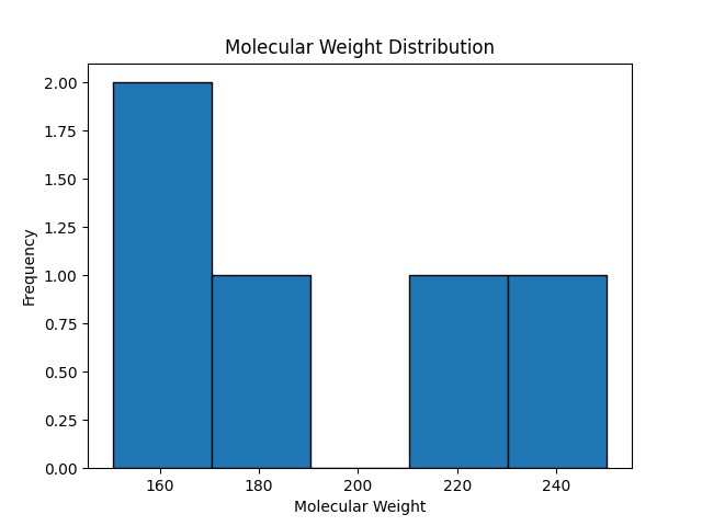
Output Explanation:

The histogram provides a clear view of how molecular weights are grouped.
The density plot shows the overall trend, highlighting where most molecular weights lie.

Practice Problem

Task:

Use the BBBP.csv dataset to explore the distribution of molecular weights.
Create a histogram and a density plot of molecular weights.
Identify the range where most molecular weights are concentrated.

▶ Show Solution Code


!pip install rdkit-pypi

# Importing packages / might have to run it twice
from rdkit import Chem
from rdkit.Chem import Descriptors
import pandas as pd
import matplotlib.pyplot as plt
import seaborn as sns

# Load the BBBP dataset
url = 'https://raw.githubusercontent.com/Data-Chemist-Handbook/Data-Chemist-Handbook.github.io/refs/heads/master/_pages/BBBP.csv'
df = pd.read_csv(url)

# Convert SMILES to molecular weight
def get_mol_weight(smile):
    mol = Chem.MolFromSmiles(smile)
    return Descriptors.MolWt(mol) if mol else None

df['MolecularWeight'] = df['smiles'].apply(get_mol_weight)

# Histogram of molecular weights
plt.hist(df['MolecularWeight'].dropna(), bins=20, edgecolor='black')
plt.title('Molecular Weight Distribution (BBBP Dataset)')
plt.xlabel('Molecular Weight')
plt.ylabel('Frequency')
plt.show()

# Density plot
sns.kdeplot(df['MolecularWeight'].dropna(), shade=True)
plt.title('Density Plot of Molecular Weight (BBBP Dataset)')
plt.xlabel('Molecular Weight')
plt.ylabel('Density')
plt.show()

Output

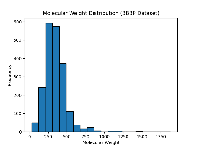
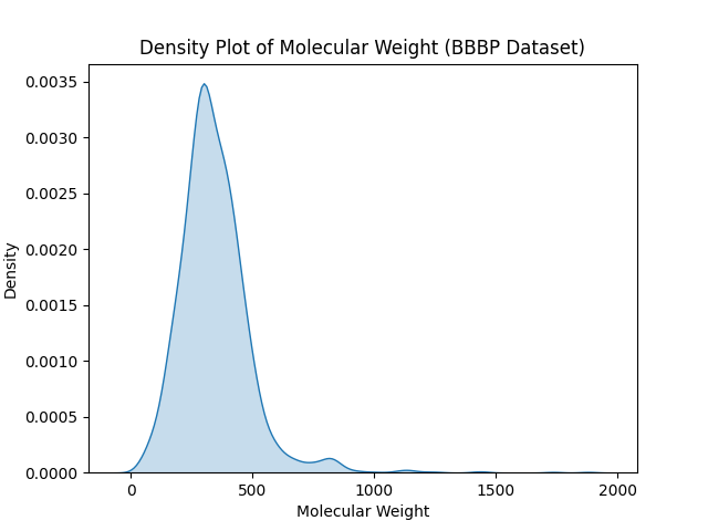
Interpretation:

The histogram provides a granular view, dividing molecular weights into discrete bins.
The density plot highlights the smooth distribution and allows chemists to identify where the majority of molecules lie.
By observing the plots, chemists can adjust dataset sampling or preprocessing steps for a balanced analysis.

Key Takeaways

Histograms are great for visualizing the frequency distribution of molecular properties.
Density plots provide a smooth view of the distribution, ideal for spotting trends.
Both tools help chemists understand their datasets, identify biases, and plan analyses effectively.

2.4.3 Similarity and Clustering

Completed and Compiled Code: Click Here

Introduction to Molecular Similarity

In cheminformatics, molecular similarity measures the resemblance between chemical structures. This concept is crucial for tasks like virtual screening, clustering, and classification of compounds. By quantifying similarity, researchers can group compounds with shared properties, predict biological activities, or identify potential drug candidates.

One common way to assess similarity is by using fingerprints—binary or hexadecimal representations of molecular features. Similarity between fingerprints is often calculated using metrics like Tanimoto similarity, which compares the overlap between two fingerprints.

Clustering in Cheminformatics

Clustering is a technique for grouping molecules based on their similarity. It helps in identifying patterns and relationships within large datasets. Two widely used clustering methods in cheminformatics are:

Hierarchical Clustering: Groups data points into a hierarchy or tree-like structure based on similarity. It provides a visual representation of relationships through a dendrogram.
K-Means Clustering: Divides data into a predefined number of clusters by minimizing the variance within each cluster. It is faster and works well for larger datasets.

Example: Fingerprints and Clustering

Let’s analyze a dataset by generating fingerprints for molecules, calculating pairwise similarity, and performing clustering.

!pip install rdkit -q

import pandas as pd
import numpy as np
from rdkit import Chem
from rdkit.Chem import rdFingerprintGenerator
from rdkit import DataStructs

data = {
    'Compound': ['Mol1', 'Mol2', 'Mol3', 'Mol4'],
    'SMILES': ['CCO', 'CCC', 'CNC', 'COC']
}
df = pd.DataFrame(data)

# Initialize Morgan fingerprint generator
generator = rdFingerprintGenerator.GetMorganGenerator(radius=2, fpSize=256)

# Generate fingerprints
fps = []
for smi in df['SMILES']:
    mol = Chem.MolFromSmiles(smi)
    if mol:
        fps.append(generator.GetFingerprint(mol))

# Compute Tanimoto similarity matrix
n = len(fps)
similarity_matrix = np.zeros((n, n))
for i in range(n):
    for j in range(n):
        similarity_matrix[i, j] = DataStructs.TanimotoSimilarity(fps[i], fps[j])

# Convert to DataFrame and print
sim_df = pd.DataFrame(similarity_matrix, columns=df['Compound'], index=df['Compound'])
print("Tanimoto Similarity Matrix:")
print(sim_df)

Output

Tanimoto Similarity Matrix:
Compound      Mol1      Mol2      Mol3      Mol4
Compound                                        
Mol1      1.000000  0.428571  0.111111  0.111111
Mol2      0.428571  1.000000  0.142857  0.142857
Mol3      0.111111  0.142857  1.000000  0.142857
Mol4      0.111111  0.142857  0.142857  1.000000

2.4.4 Regression Models for Property Prediction

Completed and Compiled Code: Click Here

Introduction to Regression Models

Regression models are essential tools in cheminformatics for predicting molecular properties, such as logP (partition coefficient), melting points, and boiling points, from other molecular descriptors. These models analyze the relationship between a dependent variable (the property being predicted) and one or more independent variables (descriptors).

Linear Regression: The simplest regression model that assumes a straight-line relationship between variables.
Multiple Regression: Extends linear regression to handle multiple predictors.
Applications in Cheminformatics: Predicting solubility, bioavailability, or toxicity from molecular properties.

By training on known data, regression models can make predictions for new molecules, assisting in drug discovery and materials design.

Example: Predicting LogP from Molecular Weight

This example demonstrates using a linear regression model to predict logP values based on molecular weight using synthetic data.

import pandas as pd
from sklearn.linear_model import LinearRegression
from sklearn.metrics import mean_squared_error, r2_score
import matplotlib.pyplot as plt

# Example dataset (synthetic data)
data = {
   'MolecularWeight': [120, 150, 180, 200, 250, 300],
   'LogP': [0.8, 1.2, 1.5, 2.0, 2.8, 3.5]
}
df = pd.DataFrame(data)

# Define independent (X) and dependent (y) variables
X = df[['MolecularWeight']]
y = df['LogP']

# Train a linear regression model
model = LinearRegression()
model.fit(X, y)

# Make predictions
predictions = model.predict(X)

# Evaluate the model
mse = mean_squared_error(y, predictions)
r2 = r2_score(y, predictions)

# Print model performance
print(f"Mean Squared Error (MSE): {mse:.2f}")
print(f"R-squared (R²): {r2:.2f}")

# Plot the data and regression line
plt.scatter(X, y, color='blue', label='Data')
plt.plot(X, predictions, color='red', label='Regression Line')
plt.xlabel('Molecular Weight')
plt.ylabel('LogP')
plt.title('Linear Regression: Molecular Weight vs LogP')
plt.legend()
plt.show()

Output

Mean Squared Error (MSE): 0.01
R-squared (R²): 0.99

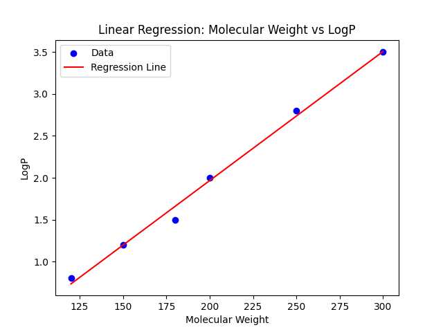
Explanation:

Data: Synthetic molecular weights and logP values are used to train the model.
Model Training: A linear regression model learns the relationship between molecular weight and logP.
Evaluation: Metrics like Mean Squared Error (MSE) and R-squared (R²) evaluate model accuracy.
Visualization: A scatter plot shows the data points and the regression line.

Practice Problem

Context: Understanding regression models is essential for predicting molecular properties. This task will help chemists apply regression models to analyze molecular data.

Task:

Create a synthetic dataset of molecular weights and melting points.
Train a linear regression model to predict melting points based on molecular weights.
Evaluate the model’s performance using MSE and R².
Visualize the data and regression line.

▶ Show Solution Code


import pandas as pd
from sklearn.linear_model import LinearRegression
from sklearn.metrics import mean_squared_error, r2_score
import matplotlib.pyplot as plt

# Example dataset (synthetic data)
data = {
   'MolecularWeight': [100, 120, 150, 180, 200, 250],
   'MeltingPoint': [50, 60, 80, 100, 110, 140]
}
df = pd.DataFrame(data)

# Define independent (X) and dependent (y) variables
X = df[['MolecularWeight']]
y = df['MeltingPoint']

# Train a linear regression model
model = LinearRegression()
model.fit(X, y)

# Make predictions
predictions = model.predict(X)

# Evaluate the model
mse = mean_squared_error(y, predictions)
r2 = r2_score(y, predictions)

# Print model performance
print(f"Mean Squared Error (MSE): {mse:.2f}")
print(f"R-squared (R²): {r2:.2f}")

# Plot the data and regression line
plt.scatter(X, y, color='green', label='Data')
plt.plot(X, predictions, color='orange', label='Regression Line')
plt.xlabel('Molecular Weight')
plt.ylabel('Melting Point')
plt.title('Linear Regression: Molecular Weight vs Melting Point')
plt.legend()
plt.show()

Output

Mean Squared Error (MSE): 1.17
R-squared (R²): 1.00

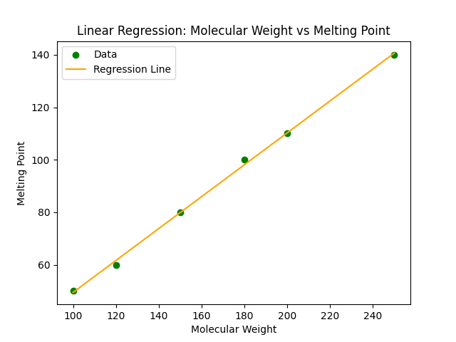
Key Takeaways

Regression models establish relationships between molecular descriptors and properties.
Linear regression is straightforward and interpretable, making it a useful first approach for property prediction.
Metrics like MSE and R² help evaluate the predictive performance of models.

2.4.5 Advanced Visualization of Representations

Completed and Compiled Code: Click Here

Introduction to Advanced Visualization

Advanced visualization techniques such as heatmaps, scatterplots, and correlation matrices provide deeper insights into molecular data by highlighting patterns and relationships. These methods are particularly useful for comparing molecular properties, identifying clusters, and understanding correlations between features.

Heatmaps: Represent data in a matrix format with color encoding to indicate values.
Scatterplots: Show relationships between two variables as points in a Cartesian plane.
Correlation Matrices: Display pairwise correlations between multiple features.

These visualizations are critical for exploring relationships in molecular data, identifying outliers, and forming hypotheses.

Heatmaps for Molecular Similarity

Heatmaps are effective for visualizing similarity matrices, which represent pairwise comparisons between molecules based on their properties or fingerprints.

import numpy as np
import seaborn as sns
import matplotlib.pyplot as plt

# Generate a synthetic similarity matrix (example data)
np.random.seed(42)
similarity_matrix = np.random.rand(5, 5)

# Create a heatmap
sns.heatmap(similarity_matrix, annot=True, cmap='coolwarm', cbar=True)
plt.title('Heatmap of Molecular Similarity')
plt.xlabel('Molecules')
plt.ylabel('Molecules')
plt.show()

Output

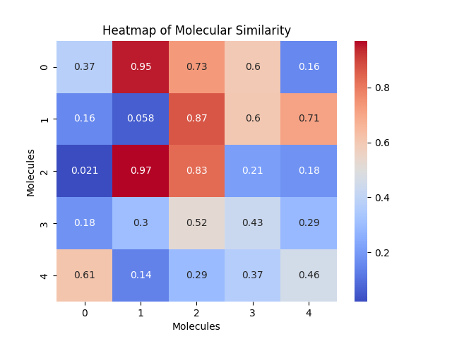
Explanation:

Data: A synthetic 5x5 similarity matrix is generated to simulate pairwise molecular comparisons.
Heatmap: The seaborn library is used to create a visually appealing heatmap.
Annotations and Color Map: Numerical values are displayed in each cell, and the coolwarm colormap enhances interpretability.

Scatterplots for Molecular Properties

Scatterplots help visualize relationships between molecular properties such as molecular weight and logP.

import pandas as pd
import seaborn as sns
import matplotlib.pyplot as plt

# Example dataset (synthetic data)
data = {
   'MolecularWeight': [100, 150, 200, 250, 300],
   'LogP': [1.0, 1.5, 2.0, 2.5, 3.0]
}
df = pd.DataFrame(data)

# Create a scatterplot
sns.scatterplot(data=df, x='MolecularWeight', y='LogP', hue='LogP', palette='viridis', size='LogP', sizes=(50, 200))
plt.title('Scatterplot of Molecular Weight vs LogP')
plt.xlabel('Molecular Weight')
plt.ylabel('LogP')
plt.legend(title='LogP')
plt.show()

Output

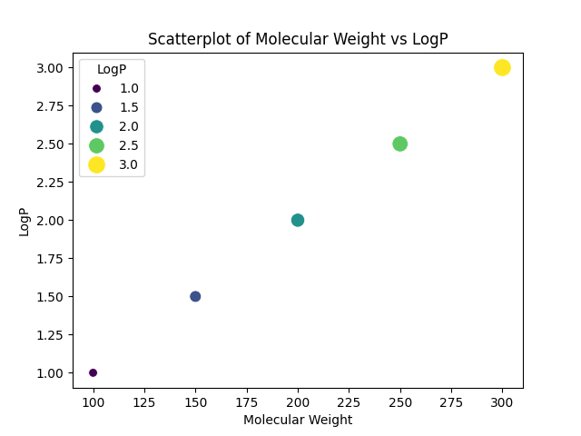
Explanation:

Data: A synthetic dataset of molecular weights and logP values is used.
Scatterplot: seaborn.scatterplot is used to add color (hue) and size (size) encoding for logP.
Interpretability: The color gradient and point sizes make it easy to identify patterns.

Correlation Matrices

Correlation matrices summarize pairwise relationships between molecular properties, highlighting strong positive or negative correlations.

import pandas as pd
import seaborn as sns
import matplotlib.pyplot as plt

# Modified example dataset with less-than-perfect correlations
data = {
    'MolecularWeight': [100, 150, 200, 250, 300],
    'LogP': [0.8, 1.4, 2.1, 2.2, 2.9],             
    'MeltingPoint': [55, 58, 72, 77, 91]            
}
df = pd.DataFrame(data)

# Calculate the correlation matrix
correlation_matrix = df.corr()

# Create a heatmap of the correlation matrix
sns.heatmap(correlation_matrix, annot=True, cmap='coolwarm', cbar=True)
plt.title('Correlation Matrix of Molecular Properties')
plt.show()

Output

Explanation:

Data: A synthetic dataset includes molecular weights, logP values, and melting points.
Correlation Matrix: Pairwise correlations between variables are calculated.
Heatmap: The matrix is visualized with seaborn.heatmap, with annotations for clarity.

Practice Problem

Context: Visualizing molecular similarity and correlations helps chemists identify patterns and relationships. This problem involves creating and interpreting heatmaps.

Task:

Generate a synthetic 6x6 similarity matrix.
Create a heatmap to visualize the similarity matrix.
Calculate a correlation matrix for molecular properties and visualize it.

▶ Show Solution Code


import numpy as np
import pandas as pd
import seaborn as sns
import matplotlib.pyplot as plt

# Generate a synthetic 6x6 similarity matrix
np.random.seed(42)
similarity_matrix = np.random.rand(6, 6)

# Create a heatmap of the similarity matrix
sns.heatmap(similarity_matrix, annot=True, cmap='Blues', cbar=True)
plt.title('Heatmap of Synthetic Molecular Similarity')
plt.xlabel('Molecules')
plt.ylabel('Molecules')
plt.show()

# Synthetic dataset of molecular properties
data = {
    'MolecularWeight': [100, 150, 200, 250, 300],
    'LogP': [0.8, 1.4, 2.1, 2.2, 2.9],             
    'MeltingPoint': [55, 58, 72, 77, 91]            
}
df = pd.DataFrame(data)

# Calculate the correlation matrix
correlation_matrix = df.corr()

# Create a heatmap of the correlation matrix
sns.heatmap(correlation_matrix, annot=True, cmap='coolwarm', cbar=True)
plt.title('Correlation Matrix of Molecular Properties')
plt.show()

Output

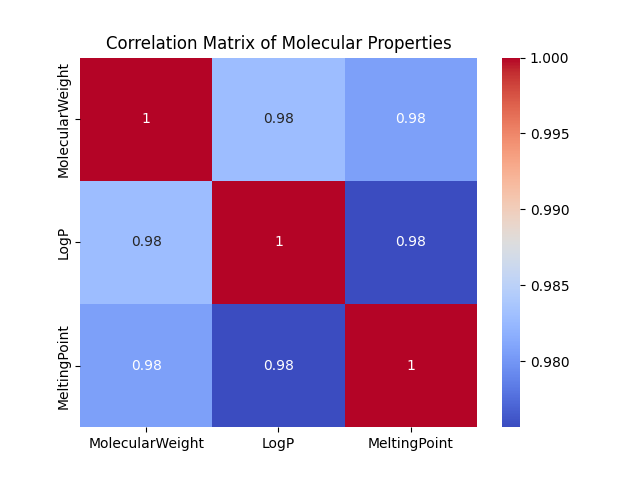
Key Takeaways

Heatmaps provide a quick overview of similarity or correlation matrices, revealing patterns and clusters.
Scatterplots visually demonstrate relationships between two molecular properties, with options for color and size encoding.
Correlation matrices highlight pairwise relationships, aiding in feature selection and hypothesis generation.

2.4.6 Integration of Representations with Machine Learning

Completed and Compiled Code: Click Here

Introduction to Integration of Representations

In cheminformatics, combining molecular representations like fingerprints, 3D coordinates, and molecular descriptors enhances the predictive power of machine learning models. These representations capture different aspects of molecular properties and behavior, providing a comprehensive dataset for prediction tasks.

Key steps in integrating representations:

Feature Extraction: Transform molecular data into numerical representations suitable for machine learning models.
Feature Combination: Combine multiple representations into a unified feature array.
Model Training: Use machine learning algorithms to train predictive models on the combined features.

This integration is critical for tasks such as property prediction, activity modeling, and virtual screening.

Combining Representations for Predictive Models

Combining fingerprints, 3D coordinates, and descriptors involves preprocessing each representation and concatenating them into a single feature array.

!pip install rdkit-pypi
from rdkit import Chem
from rdkit.Chem import AllChem, Descriptors, rdFingerprintGenerator
import numpy as np

# Example SMILES string for aspirin
smiles = 'CC(=O)OC1=CC=CC=C1C(=O)O'
molecule = Chem.MolFromSmiles(smiles)
molecule = Chem.AddHs(molecule)

# Generate fingerprint
generator = rdFingerprintGenerator.GetMorganGenerator(radius=2, fpSize=1024)
fingerprint = generator.GetFingerprint(molecule)
fingerprint_array = np.array(list(map(int, fingerprint.ToBitString())))

# Molecular descriptors
molecular_weight = Descriptors.MolWt(molecule)
logP = Descriptors.MolLogP(molecule)
descriptor_array = np.array([molecular_weight, logP])

# Generate 3D coordinates
AllChem.EmbedMolecule(molecule, randomSeed=42)
AllChem.UFFOptimizeMolecule(molecule)

# Extract 3D coordinates
conf = molecule.GetConformer()
atom_positions = []
for atom in molecule.GetAtoms():
    pos = conf.GetAtomPosition(atom.GetIdx())
    atom_positions.extend([pos.x, pos.y, pos.z])
coords_array = np.array(atom_positions)

# Combine all features
feature_array = np.concatenate((fingerprint_array, descriptor_array, coords_array), axis=None)

# Report
print(f"Molecule SMILES: {smiles}")
print(f"Number of atoms (including hydrogens): {molecule.GetNumAtoms()}")
print(f"Fingerprint length: {fingerprint_array.shape[0]}")
print(f"Number of descriptors: {descriptor_array.shape[0]}")
print(f"3D coordinate array length (flattened): {coords_array.shape[0]}")
print(f"Final feature vector shape: {feature_array.shape}")

Output

Molecule SMILES: CC(=O)OC1=CC=CC=C1C(=O)O
Number of atoms (including hydrogens): 21
Fingerprint length: 1024
Number of descriptors: 2
3D coordinate array length (flattened): 63
Final feature vector shape: (1089,)

Explanation:

Fingerprints: Encodes molecular substructures as a binary array.
Descriptors: Provides numerical values for molecular properties like molecular weight and logP.
3D Coordinates: Captures spatial arrangement, though typically preprocessed before integration.
Combination: All features are concatenated into a single array for machine learning input.

Conceptual Integration into Predictive Pipelines

Integrating representations into predictive pipelines involves preprocessing, feature engineering, and model training.

Pipeline Steps:

Data Preprocessing:
- Convert SMILES to molecular representations.
- Normalize descriptors and scale features.
Feature Engineering:
- Generate fingerprints, descriptors, and optional 3D features.
- Combine features into a unified array.
Model Training:
- Train machine learning models (e.g., Random Forest, SVM) on the combined features.
- Evaluate model performance using metrics like R², MAE, or accuracy.

Example Workflow:

Extract features from molecules using RDKit.
Combine features into arrays using NumPy.
Train a predictive model using scikit-learn.

Practice Problem

Context: Predicting molecular properties using integrated representations is a common task in cheminformatics. This problem focuses on creating feature arrays for machine learning input.

Task:

Extract fingerprints, molecular descriptors, and 3D coordinates for three molecules.
Combine these features into a single feature array for each molecule.
Print the resulting feature arrays.

▶ Show Solution Code


import numpy as np
from rdkit import Chem
from rdkit.Chem import AllChem, Descriptors, rdFingerprintGenerator

# Example SMILES strings for three molecules
smiles_list = [
   'CC(=O)OC1=CC=CC=C1C(=O)O',  # Aspirin
   'C1=CC=CC=C1',               # Benzene
   'CCO'                        # Ethanol
]

feature_arrays = []

for idx, smiles in enumerate(smiles_list):
    molecule = Chem.MolFromSmiles(smiles)
    molecule = Chem.AddHs(molecule)  # Add hydrogens

    # Generate fingerprint
    generator = rdFingerprintGenerator.GetMorganGenerator(radius=2, fpSize=1024)
    fingerprint = generator.GetFingerprint(molecule)
    fingerprint_array = np.array(list(map(int, fingerprint.ToBitString())))

    # Molecular descriptors
    molecular_weight = Descriptors.MolWt(molecule)
    logP = Descriptors.MolLogP(molecule)
    descriptor_array = np.array([molecular_weight, logP])

    # Generate 3D coordinates
    AllChem.EmbedMolecule(molecule, randomSeed=42)
    AllChem.UFFOptimizeMolecule(molecule)

    # Extract 3D coordinates
    conf = molecule.GetConformer()
    atom_positions = []
    for atom in molecule.GetAtoms():
        pos = conf.GetAtomPosition(atom.GetIdx())
        atom_positions.extend([pos.x, pos.y, pos.z])
    coords_array = np.array(atom_positions)

    # Combine all features
    feature_array = np.concatenate((fingerprint_array, descriptor_array, coords_array), axis=None)
    feature_arrays.append(feature_array)

    # Print summary
    print(f"Molecule {idx + 1}: {smiles}")
    print(f"  Number of atoms (with Hs): {molecule.GetNumAtoms()}")
    print(f"  Fingerprint length: {fingerprint_array.shape[0]}")
    print(f"  Descriptor count: {descriptor_array.shape[0]}")
    print(f"  3D coordinate length: {coords_array.shape[0]}")
    print(f"  Final feature vector shape: {feature_array.shape}\n")

# Optionally print first few values of each feature array
for i, features in enumerate(feature_arrays):
    print(f"Feature array for molecule {i + 1} (first 10 values): {features[:10]}")

Output

Molecule 1: CC(=O)OC1=CC=CC=C1C(=O)O
  Number of atoms (with Hs): 21
  Fingerprint length: 1024
  Descriptor count: 2
  3D coordinate length: 63
  Final feature vector shape: (1089,)

Molecule 2: C1=CC=CC=C1
  Number of atoms (with Hs): 12
  Fingerprint length: 1024
  Descriptor count: 2
  3D coordinate length: 36
  Final feature vector shape: (1062,)

Molecule 3: CCO
  Number of atoms (with Hs): 9
  Fingerprint length: 1024
  Descriptor count: 2
  3D coordinate length: 27
  Final feature vector shape: (1053,)

Feature array for molecule 1 (first 10 values): [0. 0. 0. 0. 0. 0. 0. 0. 0. 0.]
Feature array for molecule 2 (first 10 values): [0. 0. 0. 0. 0. 0. 0. 0. 0. 0.]
Feature array for molecule 3 (first 10 values): [0. 0. 0. 0. 0. 0. 0. 0. 0. 0.]

Key Takeaways

Integrated Representations: Combining fingerprints, descriptors, and 3D features captures multiple facets of molecular information.
Feature Engineering: Creating unified feature arrays is essential for predictive tasks.
Practical Application: These methods enable the development of robust machine learning models for cheminformatics.

Section 2.4 – Quiz Questions

Explanation: The `.mean()` method applied to a specific column in a pandas DataFrame calculates the average value for that column.

Question 5

You are working with a new dataset and would like to analyze it by making a heatmap. If you ran the following code to generate a heatmap of a similarity matrix, what would this heatmap accomplish for you in cheminformatics?

sns.heatmap(similarity_matrix, annot=True, cmap='coolwarm', cbar=True)

A. The melting point of unknown molecules.
B. The relationships between SMILES strings and IUPAC names.
C. The structural similarity between molecules based on their fingerprints.
D. The error rate in a regression model.

▶ Click to show answer

Correct Answer: C

▶ Click to show explanation

Explanation: A similarity matrix shows pairwise comparisons, often based on Tanimoto similarity, to help identify structurally similar or distinct molecules.

2) Comprehension / Application Questions

Question 6

In chemistry and data science, it may be helpful to visualize the data and understand trends within the data by creating scatter plots. In this example, imagine you want to observe the relationship between molecular weight and logP in the BBBP dataset file. Create a scatter plot with the data below to generate a scatter plot with molecular weight on the x-axis and logP on the y-axis. Make sure to label the axes appropriately.

Data:

Molecular weight: [50, 90, 134, 239, 252]
LogP: [0.7, 0.94, 1.24, 2.89, 3.21]

Which scatter plot below would look like the scatter plot you produced?

A. Answer A - Shows decreasing trend
B. Answer B - Shows no clear pattern
C. Answer C - Shows increasing trend with positive correlation
D. Answer D - Shows constant values

▶ Click to show answer

Correct Answer: C

▶ Click to show explanation

Explanation: The data shows a clear positive correlation between molecular weight and logP. As molecular weight increases from 50 to 252, logP increases from 0.7 to 3.21, indicating that larger molecules in this dataset tend to be more lipophilic.

Question 7

As a chemist analyzing a compound library, you’re interested in understanding whether larger molecules tend to be more lipophilic, which could affect their ability to cross biological membranes. You decide to use a scatter plot to explore the relationship between molecular weight and logP (a measure of lipophilicity).

Given the following code snippet:

import pandas as pd
import matplotlib.pyplot as plt

df = pd.DataFrame({
    'MolecularWeight': [180.16, 150.12, 250.23, 320.45, 200.34],
    'LogP': [2.1, 1.9, 3.5, 4.0, 2.8]
})

plt.scatter(df['MolecularWeight'], df['LogP'])
plt.xlabel('Molecular Weight')
plt.ylabel('LogP')
plt.title('Scatter Plot of Molecular Weight vs LogP')
plt.show()

What chemical insight should you expect to gain from this plot?

A. LogP decreases linearly as molecular weight increases.
B. There is no observable trend — the data is completely random.
C. LogP increases with molecular weight, suggesting a positive relationship between size and lipophilicity.
D. Molecular weight and LogP both remain constant, so no conclusion can be drawn.

▶ Click to show answer

Correct Answer: C

▶ Click to show explanation

Explanation: In this example, both molecular weight and logP increase together, suggesting that larger compounds may be more lipophilic. This kind of trend can guide medicinal chemists in optimizing drug candidates for permeability and bioavailability by balancing molecular size with lipophilicity.